Position Size Calculator - R & ATR v1# Position Size Calculator - R & ATR
Professional position sizing tool for crypto traders using risk management principles and ATR-based stop loss placement.
## Features
✅ **Automatic ATR Calculation** - Uses ATR(14) by default, customizable period
✅ **Risk Management** - Calculate position size based on portfolio % risk
✅ **Tranche Support** - Split positions into multiple entries
✅ **Visual Stop Loss** - Red line showing stop loss placement on chart
✅ **Real-time Results** - Table displays all calculations instantly
✅ **Clean Interface** - Professional table with all key metrics
## How It Works
The indicator calculates optimal position size using this formula:
1. **Risk Amount** = Portfolio Size × (Risk % / 100)
2. **Stop Distance** = ATR × Multiplier
3. **Stop Loss Price** = Entry Price - Stop Distance
4. **Position Size** = Risk Amount / Stop Distance
5. **Tranche Size** = Position Size / Number of Tranches
## Settings
**Portfolio & Risk**
- Portfolio Size (USD): Your total trading capital
- Risk per Trade (R in %): Percentage of portfolio to risk per trade
- Number of Tranches: Split position into multiple entries
**ATR Settings**
- ATR Length: Period for ATR calculation (default: 14)
- ATR Multiplier: Multiply ATR for stop loss distance (0.5x, 1x, 1.5x, etc.)
**Display**
- Show Stop Loss Line: Toggle red stop loss line on chart
- Show Calculation Table: Toggle results table
## Results Displayed
- Risk Amount (1R): Dollar amount risked on trade
- Stop Distance: Distance from entry to stop loss
- Stop Loss: Exact stop loss price
- Risk per Coin: Amount risked per unit
- Position Size (coins): Number of coins to buy
"stop loss"に関するスクリプトを検索

Smart Money Concepts [XoRonX]# Smart Money Concepts (SMC) - Advanced Trading Indicator
## 📊 Deskripsi
**Smart Money Concepts ** adalah indicator trading komprehensif yang menggabungkan konsep Smart Money Trading dengan berbagai alat teknikal analisis modern. Indicator ini dirancang untuk membantu trader mengidentifikasi pergerakan institusional (smart money), struktur pasar, zona supply/demand, dan berbagai sinyal trading penting.
Indicator ini mengintegrasikan multiple timeframe analysis, order blocks detection, fair value gaps, fibonacci retracement, volume profile, RSI multi-timeframe, dan moving averages dalam satu platform yang powerful dan mudah digunakan.
---
## 🎯 Fitur Utama
### 1. **Smart Money Structure**
- **Internal Structure** - Struktur pasar jangka pendek untuk entry presisi
- **Swing Structure** - Struktur pasar jangka panjang untuk trend analysis
- **BOS (Break of Structure)** - Konfirmasi kelanjutan trend
- **CHoCH (Change of Character)** - Deteksi potensi reversal
### 2. **Order Blocks**
- **Internal Order Blocks** - Zona demand/supply jangka pendek
- **Swing Order Blocks** - Zona demand/supply jangka panjang
- Filter otomatis berdasarkan volatilitas (ATR/Range)
- Mitigation tracking (High/Low atau Close)
- Customizable display (jumlah order blocks yang ditampilkan)
### 3. **Equal Highs & Equal Lows (EQH/EQL)**
- Deteksi otomatis equal highs/lows
- Indikasi liquidity zones
- Threshold adjustment untuk sensitivitas
- Visual lines dan labels
### 4. **Fair Value Gaps (FVG)**
- Multi-timeframe FVG detection
- Auto threshold filtering
- Bullish & Bearish FVG boxes
- Extension control
- Color customization
### 5. **Premium & Discount Zones**
- Premium Zone (75-100% dari range)
- Equilibrium Zone (47.5-52.5% dari range)
- Discount Zone (0-25% dari range)
- Auto-update berdasarkan swing high/low
### 6. **Fibonacci Retracement**
- **Equilibrium to Discount** - Fib dari EQ ke discount zone
- **Equilibrium to Premium** - Fib dari EQ ke premium zone
- **Discount to Premium** - Fib full range
- Reverse option
- Show/hide lines
- Custom colors
### 7. **Volume Profile (VRVP)**
- Visible Range Volume Profile
- Point of Control (POC)
- Value Area (70% volume)
- Auto-adjust rows
- Placement options (Left/Right)
- Width customization
### 8. **RSI Multi-Timeframe**
- Monitor 3 timeframes sekaligus
- Overbought/Oversold signals
- Visual table display
- Color-coded signals (Red OB, Green OS)
- Customizable position & size
### 9. **Moving Averages**
- 3 Moving Average lines
- Pilihan tipe: EMA, SMA, WMA
- Automatic/Manual period mode
- Individual color & width settings
- Cross alerts (MA vs MA, Price vs MA)
### 10. **Multi-Timeframe Levels**
- Support up to 5 different timeframes
- Previous high/low levels
- Custom line styles
- Color customization
### 11. **Candle Color**
- Color candles berdasarkan trend
- Bullish = Green, Bearish = Red
- Optional toggle
---
## 🛠️ Cara Penggunaan
### **A. Setup Awal**
1. **Tambahkan Indicator ke Chart**
- Buka TradingView
- Klik "Indicators" → "My Scripts" atau paste code
- Pilih "Smart Money Concepts "
2. **Pilih Mode Display**
- **Historical**: Tampilkan semua struktur (untuk backtesting)
- **Present**: Hanya tampilkan struktur terbaru (clean chart)
3. **Pilih Style**
- **Colored**: Warna berbeda untuk bullish/bearish
- **Monochrome**: Tema warna abu-abu
---
### **B. Penggunaan Fitur**
#### **1. Smart Money Structure**
**Internal Structure (Real-time):**
- ✅ Aktifkan "Show Internal Structure"
- Pilih tampilan: All, BOS only, atau CHoCH only
- Gunakan untuk entry timing presisi
- Filter confluence untuk mengurangi noise
**Swing Structure:**
- ✅ Aktifkan "Show Swing Structure"
- Pilih tampilan struktur bullish/bearish
- Adjust "Swings Length" (default: 50)
- Gunakan untuk konfirmasi trend utama
**Tips:**
- BOS = Konfirmasi trend continuation
- CHoCH = Warning untuk possible reversal
- Tunggu price retest ke order block setelah BOS
---
#### **2. Order Blocks**
**Setup:**
- ✅ Aktifkan Internal/Swing Order Blocks
- Set jumlah blocks yang ditampil (1-20)
- Pilih filter: ATR atau Cumulative Mean Range
- Pilih mitigation: Close atau High/Low
**Cara Trading:**
1. Tunggu BOS/CHoCH terbentuk
2. Identifikasi order block terdekat
3. Wait for price pullback ke order block
4. Entry saat price respek order block (rejection)
5. Stop loss di bawah/atas order block
6. Target: swing high/low berikutnya
**Color Code:**
- 🔵 Light Blue = Internal Bullish OB
- 🔴 Light Red = Internal Bearish OB
- 🔵 Dark Blue = Swing Bullish OB
- 🔴 Dark Red = Swing Bearish OB
---
#### **3. Equal Highs/Lows (EQH/EQL)**
**Setup:**
- ✅ Aktifkan "Equal High/Low"
- Set "Bars Confirmation" (default: 3)
- Adjust threshold (0-0.5, default: 0.1)
**Interpretasi:**
- EQH = Liquidity di atas, kemungkinan sweep lalu dump
- EQL = Liquidity di bawah, kemungkinan sweep lalu pump
- Biasanya smart money akan grab liquidity sebelum move besar
**Trading Strategy:**
- Wait for EQH/EQL formation
- Anticipate liquidity grab
- Entry setelah sweep dengan konfirmasi (order block, FVG, CHoCH)
---
#### **4. Fair Value Gaps (FVG)**
**Setup:**
- ✅ Aktifkan "Fair Value Gaps"
- Pilih timeframe (default: chart timeframe)
- Enable/disable auto threshold
- Set extension bars
**Cara Trading:**
1. Bullish FVG = Support zone untuk buy
2. Bearish FVG = Resistance zone untuk sell
3. Price tends to fill FVG (retest)
4. Entry saat price kembali ke FVG
5. Partial fill = valid, full fill = invalidated
**Tips:**
- FVG + Order Block = High probability setup
- Multi-timeframe FVG lebih kuat
- Unfilled FVG = strong momentum
---
#### **5. Premium & Discount Zones**
**Setup:**
- ✅ Aktifkan "Premium/Discount Zones"
- Zones akan auto-update berdasarkan swing high/low
**Interpretasi:**
- 🟢 **Discount Zone** = Area BUY (price murah)
- ⚪ **Equilibrium** = Neutral (50%)
- 🔴 **Premium Zone** = Area SELL (price mahal)
**Trading Strategy:**
- BUY dari discount zone
- SELL dari premium zone
- Avoid trading di equilibrium
- Combine dengan structure confirmation
---
#### **6. Fibonacci Retracement**
**Setup:**
- Pilih Fib yang ingin ditampilkan:
- Equilibrium to Discount
- Equilibrium to Premium
- Discount to Premium
- Toggle show lines
- Enable reverse jika perlu
- Custom colors
**Key Levels:**
- 0.236 = Shallow retracement
- 0.382 = Common retracement
- 0.5 = 50% golden level
- 0.618 = Golden ratio (penting!)
- 0.786 = Deep retracement
**Cara Pakai:**
- 0.618-0.786 = Ideal entry zone dalam trend
- Combine dengan order blocks
- Wait for confirmation candle
---
#### **7. Volume Profile (VRVP)**
**Setup:**
- ✅ Aktifkan "Show Volume Profile"
- Set jumlah rows (10-100)
- Adjust width (5-50%)
- Pilih placement (Left/Right)
- Enable POC dan Value Area
**Interpretasi:**
- **POC (Point of Control)** = Harga dengan volume tertinggi = magnet
- **Value Area** = 70% volume = fair price range
- **Low Volume Nodes** = Weak support/resistance
- **High Volume Nodes** = Strong support/resistance
**Trading:**
- POC acts as support/resistance
- Price tends to return to POC
- Breakout dari Value Area = momentum
---
#### **8. RSI Multi-Timeframe**
**Setup:**
- ✅ Aktifkan "Show RSI Table"
- Set 3 timeframes (default: chart, 5m, 15m)
- Set RSI period (default: 14)
- Set Overbought level (default: 70)
- Set Oversold level (default: 30)
- Pilih posisi & ukuran table
**Interpretasi:**
- 🟢 **OS (Oversold)** = RSI ≤ 30 = Kondisi jenuh jual
- 🔴 **OB (Overbought)** = RSI ≥ 70 = Kondisi jenuh beli
- **-** = Neutral zone
**Trading Strategy:**
1. Multi-timeframe alignment = strong signal
2. OS + Bullish structure = BUY signal
3. OB + Bearish structure = SELL signal
4. Divergence RSI vs Price = reversal warning
**Contoh:**
- TF1: OS, TF2: OS, TF3: OS + Price di discount zone = STRONG BUY
---
#### **9. Moving Averages**
**Setup:**
- Pilih MA Type: EMA, SMA, atau WMA (berlaku untuk ketiga MA)
- Pilih Period Mode: Automatic atau Manual
- Set period untuk MA 1, 2, 3 (default: 20, 50, 100)
- Custom color & width per MA
- ✅ Enable Cross Alerts
**Interpretasi:**
- **Golden Cross** = MA fast cross above MA slow = Bullish
- **Death Cross** = MA fast cross below MA slow = Bearish
- Price above all MAs = Strong uptrend
- Price below all MAs = Strong downtrend
**Trading Strategy:**
1. MA1 (20) = Short-term trend
2. MA2 (50) = Medium-term trend
3. MA3 (100) = Long-term trend
**Entry Signals:**
- Price bounce dari MA dalam trend = continuation
- MA cross dengan konfirmasi structure = entry
- Multiple MA confluence = strong support/resistance
**Alerts Available:**
- MA1 cross MA2/MA3
- MA2 cross MA3
- Price cross any MA
---
#### **10. Multi-Timeframe Levels**
**Setup:**
- Enable HTF Level 1-5
- Set timeframes (contoh: 5m, 1H, 4H, D, W)
- Pilih line style (solid/dashed/dotted)
- Custom colors
**Cara Pakai:**
- Previous high/low dari HTF = strong S/R
- Breakout HTF level = significant move
- Multiple HTF levels confluence = major zone
---
### **C. Trading Setup Combination**
#### **Setup 1: High Probability Buy (Bullish)**
1. ✅ Swing structure: Bullish BOS
2. ✅ Price di Discount Zone
3. ✅ Pullback ke Bullish Order Block
4. ✅ Bullish FVG di bawah
5. ✅ RSI Multi-TF: Oversold
6. ✅ Price bounce dari MA
7. ✅ POC/Value Area support
8. ✅ Fibonacci 0.618-0.786 retracement
**Entry:** Saat price reject dari order block dengan confirmation candle
**Stop Loss:** Below order block
**Target:** Swing high atau premium zone
---
#### **Setup 2: High Probability Sell (Bearish)**
1. ✅ Swing structure: Bearish BOS
2. ✅ Price di Premium Zone
3. ✅ Pullback ke Bearish Order Block
4. ✅ Bearish FVG di atas
5. ✅ RSI Multi-TF: Overbought
6. ✅ Price reject dari MA
7. ✅ POC/Value Area resistance
8. ✅ Fibonacci 0.618-0.786 retracement
**Entry:** Saat price reject dari order block dengan confirmation candle
**Stop Loss:** Above order block
**Target:** Swing low atau discount zone
---
#### **Setup 3: Liquidity Grab (EQH/EQL)**
1. ✅ Identifikasi EQH atau EQL
2. ✅ Wait for liquidity sweep
3. ✅ Konfirmasi dengan CHoCH
4. ✅ Order block terbentuk setelah sweep
5. ✅ Entry saat retest order block
---
### **D. Tips & Best Practices**
**Risk Management:**
- Selalu gunakan stop loss
- Risk 1-2% per trade
- Risk:Reward minimum 1:2
- Jangan over-leverage
**Confluence adalah Kunci:**
- Minimal 3-4 konfirmasi sebelum entry
- Lebih banyak konfirmasi = higher probability
- Quality over quantity
**Timeframe Analysis:**
- HTF (Higher Timeframe) = Trend direction
- LTF (Lower Timeframe) = Entry timing
- Align dengan HTF trend
**Backtesting:**
- Gunakan mode "Historical"
- Test strategy di berbagai market condition
- Record dan analyze hasil
**Market Condition:**
- Trending market = Follow BOS, use order blocks
- Ranging market = Use premium/discount zones, EQH/EQL
- High volatility = Wider stops, wait for clear structure
**Avoid:**
- Trading di equilibrium zone
- Entry tanpa konfirmasi
- Fighting the trend
- Overleveraging
- Emotional trading
---
## 📈 Recommended Settings
### **For Scalping (1m - 5m):**
- Internal Structure: ON
- Swing Structure: OFF
- Order Blocks: Internal only
- RSI Timeframes: 1m, 5m, 15m
- MA Periods: 9, 21, 50
### **For Day Trading (15m - 1H):**
- Internal Structure: ON
- Swing Structure: ON
- Order Blocks: Both
- RSI Timeframes: 15m, 1H, 4H
- MA Periods: 20, 50, 100
### **For Swing Trading (4H - D):**
- Internal Structure: OFF
- Swing Structure: ON
- Order Blocks: Swing only
- RSI Timeframes: 4H, D, W
- MA Periods: 20, 50, 200
---
## ⚠️ Disclaimer
Indicator ini adalah alat bantu analisis teknikal. Tidak ada indicator yang 100% akurat. Selalu:
- Lakukan analisa fundamental
- Gunakan proper risk management
- Praktik di demo account terlebih dahulu
- Trading memiliki resiko, trade at your own risk
---
## 📝 Version Info
**Version:** 5.0
**Platform:** TradingView Pine Script v5
**Author:** XoRonX
**Max Labels:** 500
**Max Lines:** 500
**Max Boxes:** 500
---
## 🔄 Updates & Support
Untuk update, bug reports, atau pertanyaan:
- Check documentation regularly
- Test new features in replay mode
- Backup your settings before updates
---
## 🎓 Learning Resources
**Recommended Study:**
1. Smart Money Concepts (SMC) basics
2. Order blocks theory
3. Liquidity concepts
4. ICT (Inner Circle Trader) concepts
5. Volume profile analysis
6. Multi-timeframe analysis
**Practice:**
- Start with higher timeframes
- Master one concept at a time
- Keep a trading journal
- Review your trades weekly
---
**Happy Trading! 🚀📊**
_Remember: The best indicator is your own analysis and discipline._

Strong Candle and Probability Levels Light [SYNC & TRADE]Indicator Description: "Strong Candle and Probability Levels Light "
Core Philosophy: This indicator is not just a collection of random signals. It is a complete trading system built around two core concepts: Strength (Volume-based Candles) and Probability (Fibonacci Levels), synchronized between spot and futures markets to filter out noise and manipulations.
🎯 The "Strong Candle Defense" Strategy
The primary tactic is to enter in the direction of the market's dominant force at an optimal price.
1. Identifying Strength: The indicator identifies "Strong Candles" in real-time — candles with anomalously high volume and significant delta (buyer/seller dominance), confirmed across multiple timeframes. They are marked with circles (blue for bullish, red for bearish) and Z-level labels showing the statistical significance of the move.
2. "Ladder" Entry: We do not chase the market. The strategy is to wait for a pullback (retest) to the body of the strong candle or its key internal Fibonacci levels (38.2%, 50%, 61.8%) for a favorable entry. The position is built in parts ("scaling in") as the bounce is confirmed.
3. Profit-Taking Targets: The main take-profit targets are set at the external Fibonacci extension levels:
First Target: 161.8% — The classic level to secure the first portion of profits.
Second Target: 261.8% (or 227% in Light mode) — The level for capturing extended moves, where the remaining position is exited.
Refined Stop-Loss Rules and Strategy Invalidation Conditions:
Primary Stop-Loss: Placed beyond the extreme of the strong candle (the Fibonacci grid's 0% level). For a long position — below the strong candle's low; for a short position — above its high.
Strategy Invalidation Criterion: The strategy is considered invalidated, and the position should be exited, if the price closes a candle's body beyond the key protective level. This specifically means:
For a Long: A candle closes (the close price) below the low of the strong candle.
For a Short: A candle closes (the close price) above the high of the strong candle.
This criterion, especially on lower timeframes, provides a stricter and more timely signal of a setup failure than a mere wick break.
Alternative Supertrend Stop-Loss: The proprietary Supertrend line can be used as a dynamic trailing stop. The stop-loss is placed behind the Supertrend line, and a candle close beyond this line also signals a trend violation and the need to exit the position.
📊 Unique Automated Fibonacci Grids
Our Fibonacci grids are not the standard, static drawing tool. They are a dynamic profit-taking and management system.
Automatic Plotting: A new grid is automatically drawn on every new strong candle, freeing the trader from manual work.
Smart Management:
Self-Cleaning: When enabled, the grid automatically removes itself after the price has fully "filled" its range (reached the 0% level), preventing chart clutter.
Dynamic Levels: Depending on the selected type (Fibonacci Light, Standard, Extended, Geometric), a different set of internal and external levels is plotted, adapting the tool to various trading styles from scalping to position trading.
Key Difference from Standard Tools: Unlike the basic Fibonacci tool, our grids are an integral part of the trading logic. They are tied to strong candles (high-probability points), update automatically, and act as an execution system for the strategy, not just an analysis tool.
📈 Proprietary Supertrend with Advanced Filtering
We do not use the standard, off-the-shelf Supertrend. Our version is a hybrid algorithm, supercharged with volume analysis.
Dynamic ATR Multiplier: The indicator's multiplier adapts to market conditions. During high volume delta (strong buying/selling pressure), the multiplier increases, making the trend line less sensitive and helping you stay in the trade during strong impulses.
Strong Candle Filter: Supertrend signal changes can be optionally restricted to confirm only on strong candles. This drastically reduces false entries. The trend doesn't change just based on volatility (ATR), but upon confirmation by real strength (volume).
Profit Potential: Combining signals from this filtered Supertrend with the "Strong Candle Defense" strategy allows for precise entry timing in the direction of the major trend, with clear and statistically sound profit targets.
⚙️ Additional Systems for Enhanced Accuracy
Spot & Futures Sync: The indicator compares strength between spot and futures markets. A divergence (e.g., a strong long candle on spot but weakness on futures) is marked as a potential "Manipulation" (X), warning you of an unreliable signal.
Multi-Timeframe Volume Analysis: Delta and volume are analyzed from lower timeframes, providing a more granular picture within a single candle of your current TF.
Supertrend Table: A quick overview of the trend direction across all major timeframes (from 5m to 1W) in a single table.
Conclusion:
The "Strong Candle and Probability Levels Light" indicator is a professional suite for traders who want to trade not just signals, but probabilities. The strategy, built around defending strong candles, combined with unique automated Fibonacci grids and an adaptive Supertrend, provides a clear plan from entry to exit. The use of market synchronization and multi-timeframe volume analysis minimizes noise and false signals, allowing you to focus on high-quality setups.

Turtle Long & Short (Donchian + N-Stop). Overview and Core Functionality
The indicator implements the classic Turtle Trading System rules. It uses two sets of Donchian Channels for generating entry and exit signals, and the Average True Range (ATR), referred to as N, to calculate a dynamic, volatility-adjusted initial stop-loss.
The script simulates a position's life cycle (entry, holding the fixed initial stop, and exiting) and only conditionally displays the calculated initial stop-loss price on the chart when a trade signal is active.
2. Key Input Parameters (Adjustable Settings)
The script provides detailed input groups for customization:
A. Signal Settings:
len_entry (Default: 20): Period for the Entry Donchian Channel (20-day high/low breakout).
len_exit (Default: 10): Period for the Exit Donchian Channel (10-day low/high trailing stop).
B. Risk Settings (N):
len_atr (Default: 20): Period used to calculate the Average True Range (N), which determines volatility.
stop_loss_multiplier (Default: 2.0): The factor applied to N to calculate the initial stop-loss (e.g., 2.0×N=2N).
C. Label Display: Controls the appearance of the entry labels.
label_background_color_long / label_background_color_short: Background color for Long/Short entry labels.
label_text_color: Text color for the labels.
label_size_input: Size control for the label (tiny, small, normal, large, huge).
3. Trading Logic and State Management
A. Entry and Exit Conditions
Trade Type Entry Condition Trailing Exit Condition Stop-Loss (SL)
Long Close > 20-period High Close < 10-period Low Fixed Entry Price−(Multiplier×N)
Short Close < 20-period Low Close > 10-period High Fixed Entry Price+(Multiplier×N)
In Google Sheets exportieren
B. Position State Management
The script uses persistent var float variables (fixed_long_stop_price and fixed_short_stop_price) to maintain the state:
Upon an Entry signal, the calculated stop-loss price is fixed and assigned to the respective var variable.
The variable holds this fixed price on subsequent bars.
The price is reset to na (Not Applicable) only when an Exit condition (10-period trailing exit, fixed stop-loss hit, or reverse entry signal) is met.
This logic ensures the initial stop-loss line is plotted only when a simulated trade is active.
4. Visual Elements and Alerts
Donchian Channels: Plotted as two lines (Entry High/Exit Low) with a fill for visualization.
N-Stop-Loss Lines: Two lines (fixed_long_stop_price in Fuchsia and fixed_short_stop_price in Orange) are plotted using plot.style_linebr, ensuring they appear only after a trade signal fires and disappear on exit.
Signal Shapes (plotshape):
Long Entry: Green triangle below the bar.
Short Entry: Red triangle above the bar.
Long/Short Exits: Diamond shapes indicating the trailing stop exit.
Entry Labels (label.new): Custom-colored labels appear at the point of entry, displaying the current N value and the exact calculated N-Stop price.
Alerts (alertcondition): Alerts are set up for both Long Entry and Short Entry conditions.

Cumulative Delta_Effort vs Result_immy**Cumulative Delta Oscillator\_effort**
This script creates a “Cumulative Delta Effort vs Result” oscillator, a custom indicator designed to measure the balance between buying and selling pressure (Effort) versus actual price movement (Result).
**How It Works**
Delta Volume: Measures aggressive buying vs selling per candle.
Cumulative Delta: Tracks net buying/selling pressure over time.
Effort vs Result: Compares volume delta (effort) to price movement (result).
Oscillator: Highlights divergence between effort and result, useful for spotting absorption (high effort, low result) and exhaustion (low effort, high result).
Histogram: Visual cue for accumulation/distribution zones.
----------------------------
This indicator combines volume delta (effort) and price movement (result), so it tells you how efficiently volume is moving price — a concept sometimes called effort vs. result analysis in Wyckoff or volume–spread analysis (VSA).
🔍 Concept Summary
Effort (delta volume) = how much buying/selling pressure is there (volume side).
Result (price change) = how much that effort moves price (price side).
Oscillator (Effort − Result) = how much “extra” effort is not producing movement — often showing absorption or exhaustion.
📈 How to Interpret the Signals
1\. Oscillator above Signal line → Bullish Momentum
When osc > signal, histogram turns green.
Means buying effort is stronger than price reaction — often early sign of accumulation or rising demand.
This can signal:
Possible bullish continuation if confirmed by rising prices.
Or early absorption if prices aren’t yet breaking out (smart money absorbing supply).
✅ Bullish Entry Signal:
When the oscillator crosses above the signal line (green cross) and price is near support or consolidating → potential long setup.
2\. Oscillator below Signal line → Bearish Momentum
When osc < signal, histogram turns red.
Selling effort dominates; can mean increasing supply or price exhaustion.
This often appears before:
Bearish continuation (trend strengthening)
Or upthrust/exhaustion (price rising on weak volume)
❌ Bearish Entry Signal:
When the oscillator crosses below the signal line (red cross), especially if near resistance → potential short setup.
3\. Crossovers
The alert is triggered when: ta.cross(osc, signal)
That means:
Bullish crossover: oscillator line crosses above signal → potential buy momentum shift.
Bearish crossover: oscillator line crosses below signal → potential sell momentum shift.
These work like MACD crossovers, but volume-adjusted.
4\. Zero Line
The zero line is the neutral point.
When osc crosses above zero, overall buying effort exceeds price change — market gaining strength.
When osc crosses below zero, selling pressure increases — market weakening.
→ Combining signal line crosses with zero-line crosses gives stronger confirmation.
5\. Histogram Analysis (Absorption \& Exhaustion)**
Tall green bars: rising momentum (buyers dominate)
Tall red bars: falling momentum (sellers dominate)
Shrinking bars: momentum fading — possible reversal zone.
If volume increases but price stalls, oscillator may spike while price stays flat — absorption (big players taking the opposite side).
If price surges but oscillator weakens, exhaustion — move running out of volume support.
------------------------------------------------------------------------
🧠 Practical Strategy Example
Situation What It Might Mean Possible Action
Oscillator crosses above signal near support Buyer effort increasing, price may rise Go long / close shorts
Oscillator crosses below signal near resistance Seller effort rising, price may drop Go short / take profits
Oscillator high but price flat Absorption (big players absorbing supply) Wait for breakout confirmation
Oscillator low but price flat Absorption (demand absorbing supply) Look for bullish reversal
Oscillator diverges from price Volume–price divergence Early warning of reversal
⚙️ Best Practice
Works best on volume-sensitive assets (futures, crypto, forex tick data).
**Combine with:**
Price structure (support/resistance)
Volume profile / delta footprint
Candle confirmation
We’ll go through both bullish and bearish examples so you can see how to trade with it in real market context.
---------------------------------------------------------------------------------
🟩 Example 1 — Bullish Setup (Long Trade)
Step 1. Context: Identify Potential Support Zone
Before relying on any indicator, find support using:
Previous swing low
Demand zone
VWAP / volume profile node
Trendline or moving average
👉 You’re looking for a place where buyers might step in.
Step 2. Wait for Oscillator Signal
Watch the oscillator panel:
The oscillator (green line) has been below the signal line (orange) → bearish phase.
Then it crosses above the signal line and the histogram turns green.
This means:
➡️ Buying “effort” is increasing faster than price reaction — momentum shift upward.
Step 3. Confirm with Price
On your chart:
Candle closes above short-term resistance or above previous candle high
Ideally volume confirms (green candle with increasing volume)
✅ Bullish Entry Condition
osc crosses above signal
price closes above local resistance
Step 4. Entry \& Stop
Entry: Next candle open after confirmation cross
Stop-loss: Below recent swing low or support zone
Take profit:
2R or 3R target
or near next resistance level
🧠 Optional filter: Only take the trade if oscillator is rising from below zero (coming out of weakness).
Step 5. Manage Trade
If oscillator flattens or starts curling down → tighten stop
If it crosses below the signal again → consider exit
Example Interpretation:
Oscillator crosses above signal from -200 to +100, histogram turns green, price breaks a resistance line → strong bullish reversal → enter long.
🟥 Example 2 — Bearish Setup (Short Trade)
Step 1. Context: Find Resistance
Look for: Prior swing high
Supply zone
Major moving average
Trendline top
Step 2. Wait for Oscillator Cross Down
The oscillator (green) crosses below the signal line (orange).
Histogram turns red.
This means:
➡️ Selling effort is rising relative to price movement — bearish pressure.
Step 3. Confirm with Price
Price fails to make higher highs, or
Forms a bearish engulfing candle near resistance.
✅ Bearish Entry Condition
osc crosses below signal
price confirms with bearish candle
Step 4. Entry \& Stop
Entry: On next candle open
Stop-loss: Above resistance or recent swing high
Take profit: 2R or more or at next major support
Step 5. Exit on Opposite Signal
If oscillator crosses back above signal → momentum shift → exit short.
⚙️ Pro Tips
Tip Why It Matters
Use on 15m–4H+ charts More reliable delta signal
Combine with volume or OBV Confirms “effort” strength
Watch divergences Early reversals
Align with higher timeframe trend Avoid countertrend traps
-------------------------------------------------------------------------------------------------
🧩 Quick Checklist
Step Condition Action
1 Identify zone (support/resistance) Mark area
2 Oscillator crossover Prepare order
3 Candle confirmation Enter
4 Stop-loss \& target Manage risk
5 Opposite cross Exit
Please follow and like if you appreciate my work. thank you.

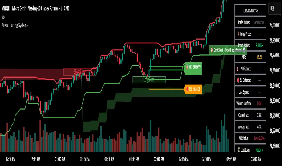
Pulsar Trading System-LITE📡 Pulsar Trading System
OVERVIEW
Pulsar is a comprehensive breakout trading system that combines dynamic support/resistance detection, trend filtering, and volume confirmation to identify high-probability entry opportunities. Unlike simple breakout indicators, Pulsar uses multi-timeframe analysis and adaptive ATR-based calculations to filter false signals and provide complete trade management from entry to exit.
WHAT MAKES THIS ORIGINAL
This indicator is unique in its integration of multiple complementary systems:
-Adaptive ATR Zones: Support and resistance levels are not static—they dynamically adjust based on current market volatility (ATR), creating entry zones that expand and contract with market conditions rather than using fixed price levels.
-Multi-Timeframe SuperTrend Filter: The trend filter operates on a higher timeframe than the chart (e.g., 5-minute SuperTrend on a 1-minute chart) to prevent counter-trend trades while maintaining granular entry precision. The visual ribbon with humorous warning text ("🚫 Don't Short - Trend is Your Friend! 📈") provides immediate trend awareness.
-Intelligent Cooldown System: After any trade exit (stop loss or take profit), the system enters a configurable cooldown period, preventing overtrading during choppy or consolidating market conditions—a critical feature often missing in breakout systems.
-Dynamic Trailing Stops: The trailing stop uses ATR multipliers to lock in profits while adapting to volatility, moving only in the favorable direction and never loosening.
-Comprehensive Dashboard: Real-time analysis displays trade status, entry prices, distances to targets in both points and ATR multiples, volume confirmation status, and cooldown countdown.
HOW IT WORKS
Core Detection Logic:
Pulsar identifies breakout opportunities by monitoring price interaction with dynamically calculated support and resistance levels:
Support/Resistance Calculation: Uses ta.lowest() and ta.highest() over a configurable lookback period to identify key levels, then adds ATR-based buffers (0.5 × ATR) to create entry zones.
Breakout Conditions:
Long Entry: Price closes above support buffer AND recent low touched support AND volume exceeds threshold
Short Entry: Price closes below resistance buffer AND recent high touched resistance AND volume exceeds threshold
SuperTrend Filter: A separate higher-timeframe SuperTrend calculation determines overall trend direction. Entries only trigger when breakout direction aligns with SuperTrend (bullish breakout + bullish trend, or bearish breakout + bearish trend).
Volume Confirmation: Current volume must exceed a configurable multiple of the 14-period SMA (default 1.0×) to confirm genuine interest in the breakout.
Cooldown Mechanism: After exit, the system tracks bars elapsed and blocks new signals until the cooldown period completes, preventing rapid-fire entries in ranging markets.
Trade Management:
Stop Loss: Calculated as entry zone ± (ATR × SL Multiplier)
Take Profit 1: Entry zone ± (ATR × TP1 Multiplier)
Take Profit 2: Entry zone ± (ATR × TP2 Multiplier)
Trailing Stop (optional): Updates every bar, moving the stop closer by maintaining distance of (ATR × Trailing Multiplier) from current price, but only in favorable direction
SuperTrend Calculation:
The SuperTrend uses standard methodology:
Upper Band = (High + Low) / 2 + (Multiplier × ATR)
Lower Band = (High + Low) / 2 - (Multiplier × ATR)
Direction changes when price crosses opposite band
The ribbon visualization adds a width offset (ATR × Ribbon Width) to create a filled zone rather than a single line.
HOW TO USE
Setup:
Add Pulsar to your chart (works best on liquid instruments like NQ, ES, CL)
Configure timeframe-specific settings (see recommendations below)
Enable SuperTrend Filter for trend-following mode, or disable for pure breakout mode
Set up alerts for Entry, TP1, TP2, and Stop Loss events
Recommended Settings by Timeframe:
1-Minute Charts:
Lookback Period: 10-15
SuperTrend Timeframe: 5 min
ATR Timeframe: 5 min (for stability)
Cooldown: 8-12 bars
Trailing Stop: Enabled with 0.8-1.0 multiplier
5-Minute Charts:
Lookback Period: 15-20
SuperTrend Timeframe: 15 min
ATR Timeframe: current chart
Cooldown: 5-8 bars
Trailing Stop: Optional
15-Minute+ Charts:
Lookback Period: 20-30
SuperTrend Timeframe: 1 hour
ATR Timeframe: current chart
Cooldown: 3-5 bars
Trailing Stop: Optional
Interpreting Signals:
Long/Short Zone Box: Green (long) or red (short) box appears when breakout conditions are met
Blue Entry Line: Shows your entry price
Red/Orange SL Line: Red = fixed stop, Orange = trailing stop (moves in real-time)
Green TP Lines: TP1 (closer) and TP2 (further) targets
SuperTrend Ribbon: Green = bullish trend (favor longs), Red = bearish trend (favor shorts)
Dashboard Status: Monitor trade state, distances, volume confirmation, and cooldown
Best Practices:
Use SuperTrend Filter: Significantly reduces false signals by avoiding counter-trend trades
Enable Cooldown on Fast Timeframes: Prevents overtrading on 1-5 minute charts
Volume Confirmation is Critical: Don't lower volume multiplier below 0.9 on futures
Use Higher Timeframe ATR: On 1-minute charts, use 5-minute ATR for stability
Avoid Major News Events: Disable during FOMC, NFP, CPI releases
Scale Out Strategy: Consider taking partial profits at TP1, letting remainder run to TP2
Parameter Optimization:
Start conservative and adjust based on results:
Too many stop-outs: Increase SL multiplier or SuperTrend multiplier
Missing good trades: Decrease volume multiplier or cooldown period
Too many false signals: Increase volume multiplier, lookback period, or cooldown
Profits not protected: Enable trailing stop or reduce trailing multiplier
KEY FEATURES
✅ Dynamic ATR-Based Zones: Entry, stop loss, and take profit levels automatically adjust to market volatility
✅ Multi-Timeframe Trend Filter: Uses higher timeframe SuperTrend to eliminate counter-trend trades
✅ Volume Confirmation: Filters low-volume false breakouts
✅ Intelligent Cooldown: Prevents overtrading with configurable post-trade waiting period
✅ Trailing Stop System: Optional dynamic stops that lock in profits using ATR distance
✅ Real-Time Dashboard: 13-row analysis showing trade status, targets, distances, volume, and cooldown
✅ Visual Ribbon Warnings: Humorous trend-following reminders on SuperTrend ribbon
✅ Complete Alert System: Notifications for entries, TP1, TP2, fixed stops, and trailing stops
✅ Customizable Visuals: Adjustable colors, dashboard position, text size, and line lengths
✅ Non-Repainting: Uses lookahead = barmerge.lookahead_off for all multi-timeframe calculations
SETTINGS EXPLAINED
SuperTrend Filter:
Enable: Toggle trend filtering on/off
Timeframe: Higher timeframe for trend analysis (recommended 3-5x chart timeframe)
ATR Period: Period for ATR calculation in SuperTrend (10-14 standard)
Multiplier: Distance from center band (2.5-3.5 for most markets)
Ribbon Width: Visual thickness of trend ribbon (0.2-0.5)
Core Parameters:
Lookback Period: Bars used to identify support/resistance (lower = more sensitive)
ATR Period: Bars for Average True Range calculation (14 is standard)
ATR Timeframe: Use higher timeframe ATR for smoother calculations on fast charts
Volume Multiplier: Required volume vs average (1.0 = average, 1.5 = 50% above average)
TP/SL:
SL Multiplier: Stop loss distance in ATR units (1.0-2.0 typical)
TP1 Multiplier: First target in ATR units (1.5-2.5 typical)
TP2 Multiplier: Second target in ATR units (2.0-3.5 typical)
Trailing Stop:
Enable: Activate dynamic trailing stop
Multiplier: Distance from current price in ATR units (0.8-1.5 typical)
Cooldown:
Enable: Prevent new signals after trade exit
Bars: Number of bars to wait before allowing next trade (higher on fast timeframes)
IMPORTANT NOTES
⚠️ Not a Holy Grail: No indicator is perfect. Pulsar is a tool that requires proper risk management, position sizing, and trading discipline.
⚠️ Backtest First: Test settings on historical data before live trading. Results vary by instrument, timeframe, and market conditions.
⚠️ Market Conditions Matter: Breakout systems perform best in trending markets. Consider reducing size or disabling during known choppy periods.
⚠️ Stop Loss is Mandatory: Always use the provided stop loss levels. Markets can move against you rapidly.
⚠️ Volume Data Required: This indicator requires volume data to function properly. It will display a warning if volume is unavailable.
⚠️ No Repainting: All multi-timeframe calls use non-repainting settings. What you see in real-time is what will be plotted historically.
TECHNICAL SPECIFICATIONS
Version: Pine Script v6
Type: Indicator (overlay = true)
Max Boxes: 500 (for zone visualization)
Max Lines: 500 (for TP/SL levels)
Max Labels: Unlimited (for annotations)
Repainting: None (uses lookahead = barmerge.lookahead_off)
COMPATIBLE INSTRUMENTS
Works best on liquid instruments with reliable volume data:
✅ Futures: NQ, MNQ, ES, MES, YM, MYM, RTY, M2K, CL, GC
✅ Forex: Major pairs (EUR/USD, GBP/USD, etc.)
✅ Stocks: Large-cap stocks with high volume
⚠️ Crypto: Works but requires higher ATR multipliers
❌ Low Volume Stocks: May produce unreliable signals
SUPPORT
For questions, suggestions, or to report issues, please comment below. I actively maintain this indicator and appreciate feedback from the community.
Enjoy trading with Pulsar! 🌟
Smart Liquidity & OTE Analysis Tool # Smart Liquidity & OTE Analysis Tool
## OVERVIEW
This indicator is designed for traders who utilize institutional trading concepts, specifically liquidity sweeps and optimal trade entry (OTE) zones, combined with session-based market structure analysis. It identifies potential market manipulation points where stop losses are likely clustered, and highlights high-probability entry zones based on Fibonacci retracements.
The tool combines four main analytical components that work synergistically to identify trading opportunities aligned with smart money behavior.
---
## CORE CONCEPTS & METHODOLOGY
### 1. TRADING SESSIONS ANALYSIS
**What it does:**
The indicator tracks three major forex trading sessions with customizable time zones:
- **Asian Session** (Default: 01:00-13:00 UTC+4) - Typically characterized by range-bound price action
- **London Session** (Default: 11:00-20:00 UTC+4) - High volatility period with increased institutional activity
- **New York Session** (Default: 17:00-00:00 UTC+4) - Overlaps with London creating peak liquidity
**How it works:**
- Automatically highlights active sessions with colored background boxes
- Draws session high/low lines which often act as intraday support/resistance
- Identifies session overlaps (e.g., London-NY overlap) where volatility and liquidity are highest
- Color-codes the price bars during overlaps to alert traders to increased opportunity periods
- Displays real-time session status (🟢 Open / 🔴 Closed) for quick reference
**Trading Application:**
Session highs and lows frequently become liquidity targets. The indicator helps traders anticipate when price might sweep these levels before continuing in the original direction. Session overlaps are prime times for major moves as multiple institutional players are active simultaneously.
---
### 2. EXTERNAL LIQUIDITY SWEEPS
**What it does:**
Identifies when price "sweeps" or breaks beyond significant swing highs and lows where stop losses are typically clustered. These sweeps often precede reversals or continuations after liquidity is collected.
**How it works:**
- Scans the previous 20 bars (configurable) to identify swing high and low points
- Marks these levels as "buyside liquidity" (above highs) or "sellside liquidity" (below lows)
- Monitors price action using three detection methods:
* **Wick Break:** Any candle wick extending beyond the liquidity level
* **Close Break:** Candle body closing beyond the level (stronger confirmation)
* **Full Retrace:** Price breaks the level then closes back inside the range (classic liquidity grab)
- Uses an ATR-based buffer to avoid false signals from minor price spikes
- Confirms sweeps only after a configurable number of confirmation bars to reduce repainting
**The Logic Behind It:**
Institutional traders need liquidity to fill large orders. Stop losses clustered above swing highs and below swing lows provide this liquidity. When these levels are swept, it often indicates smart money is entering positions in the opposite direction, causing reversals.
**Visual Representation:**
- Blue horizontal lines mark buyside liquidity zones (above price)
- Gray horizontal lines mark sellside liquidity zones (below price)
- Labels indicate when liquidity has been swept (✓) or remains active
- Historical zones are maintained for context (configurable display limit)
---
### 3. INTERNAL LIQUIDITY DETECTION
**What it does:**
Identifies equal highs (EQH) and equal lows (EQL) within recent price action - levels that have been tested multiple times without breaking. These represent internal liquidity pools that price often revisits before making larger moves.
**How it works:**
- Examines the most recent 8 bars (configurable) for price levels that occur multiple times
- Uses an ATR-based threshold (default 0.1% of ATR) to determine if highs or lows are "equal"
- Requires minimum 3 occurrences (configurable) of the same level to qualify as internal liquidity
- Tracks both the creation and sweeping of these internal levels
- Differentiates between wick breaks and close breaks for sweep confirmation
**The Concept:**
Unlike external liquidity at swing points, internal liquidity represents recent stop clusters and pending orders within the current price structure. Identifying these levels helps traders anticipate short-term price targets and potential reversal points before larger directional moves.
**Why This Matters:**
Price often needs to clear internal liquidity before making sustained moves to external liquidity levels. This creates a "roadmap" of where price is likely to go in sequence, improving trade timing.
**Visual Representation:**
- Cyan lines mark internal buyside liquidity (equal highs)
- Orange lines mark internal sellside liquidity (equal lows)
- Dashed or solid lines based on user preference
- Labels show when internal levels are swept
---
### 4. OPTIMAL TRADE ENTRY (OTE) ZONES
**What it does:**
Calculates and displays Fibonacci retracement zones (0.618-0.786) from recent swing points, representing "discount" or "premium" areas where institutional traders often enter positions after a liquidity sweep or structure break.
**How it works:**
- Identifies swing highs and lows using a 10-bar lookback period (configurable)
- Calculates three key Fibonacci levels:
* **0.618** - The "golden ratio" retracement (most significant)
* **0.705** - Mid-point between 0.618 and 0.786
* **0.786** - Deep retracement level (square root of 0.618)
- Optionally requires a structure break before displaying OTE zones
- Dynamically extends zones as new price action develops
- Tracks whether price has entered the zone (✅) or exited without filling (❌)
- Displays up to 2 most recent zones (configurable) to avoid chart clutter
**The Methodology:**
OTE zones represent areas where price is at a "discount" (for longs) or "premium" (for shorts) relative to the recent swing. After a liquidity sweep or structure break, institutional traders often wait for retracements into these zones before entering, as it offers better risk-to-reward ratios.
**Combining with Liquidity:**
The most powerful setups occur when:
1. External liquidity is swept
2. Price retraces into an OTE zone
3. Internal liquidity is present as a target
This confluence suggests smart money activity and high-probability trade opportunities.
**Visual Representation:**
- Shaded blue zone between 0.618 and 0.786 levels
- Three horizontal lines showing key Fibonacci levels with different colors/styles
- Labels (🎯) indicate bullish or bearish OTE zones
- Entry (✅) and exit (❌) status for each zone
---
## WHY THESE FEATURES WORK TOGETHER
This indicator combines these four components because they represent different stages of institutional trading behavior:
1. **Session Timing** - Identifies WHEN institutional activity is highest
2. **Liquidity Sweeps** - Shows WHERE smart money is collecting liquidity
3. **OTE Zones** - Highlights WHERE institutional entries likely occur after sweeps
4. **Internal Liquidity** - Provides SHORT-TERM targets for profit-taking or add-ons
Rather than using each concept in isolation, this integration creates a complete market structure framework. For example:
- A buyside liquidity sweep during London open →
- Followed by a retrace into a bullish OTE zone →
- With internal sellside liquidity as the initial target
This sequence represents a complete high-probability trade setup aligned with smart money principles.
---
## ANTI-REPAINTING FEATURES
**The Repainting Problem:**
Many indicators that identify patterns on historical data repaint their signals when live trading, showing signals that weren't actually there in real-time. This creates a false sense of accuracy.
**Our Solution:**
- **Confirmation Bars Setting:** Signals only appear after X bars have confirmed the pattern (default: 2 bars)
- **Marked Confirmation:** Labels show "C" when using confirmed signals
- **Trade-off:** More confirmation = less repainting but slightly delayed signals
- **User Control:** Traders can toggle between real-time signals (faster but may repaint) and confirmed signals (delayed but reliable)
---
## KEY CUSTOMIZATION OPTIONS
### Master Controls
- Toggle each major feature on/off independently
- Combine only the features relevant to your trading style
### Display Settings
- Adjust lookback periods for each component
- Control number of historical zones displayed
- Customize colors, line styles, and transparency
- Show/hide labels and session names
- Configure text sizes for different screen setups
### Detection Sensitivity
- **Sweep Detection:** Choose between wick breaks, close breaks, or full retraces
- **ATR Buffer:** Add distance requirements to confirm sweeps (reduces false signals)
- **Equal Level Threshold:** Adjust how close levels must be to qualify as "equal"
- **Confirmation Bars:** Balance between signal speed and reliability
### Alert System
- Session open/close notifications
- Liquidity sweep alerts
- OTE zone entry alerts
- Configurable alert frequency and types
---
## HOW TO USE THIS INDICATOR
### Basic Setup
1. Add the indicator to your chart (works on all timeframes, though 5M-1H recommended for intraday)
2. Enable the features you want to use via Master Controls
3. Adjust colors and transparency to match your chart preferences
4. Configure alert preferences if using notifications
### Trading Workflow
**Step 1: Identify the Session**
- Determine which trading session is active or approaching
- Note session highs/lows as potential liquidity targets
- Be especially alert during session overlaps
**Step 2: Watch for Liquidity Sweeps**
- Monitor external liquidity lines (swing highs/lows)
- When price sweeps liquidity, anticipate a potential reversal
- Stronger sweeps (close breaks + full retraces) are more significant
**Step 3: Wait for OTE Retracement**
- After a sweep, wait for price to retrace into the OTE zone (0.618-0.786)
- Bullish OTE after sellside sweep = potential long
- Bearish OTE after buyside sweep = potential short
**Step 4: Use Internal Liquidity as Targets**
- Look for internal liquidity in the direction of your trade
- These serve as initial profit targets
- External liquidity serves as extended targets
**Step 5: Manage Confirmation Settings**
- For live trading, use confirmed signals (2+ confirmation bars)
- For backtesting or analysis, you may use real-time signals
- Note that confirmed signals appear with "C" marking
### Example Trade Scenarios
**Bullish Setup:**
1. London session opens (increased volume)
2. Price sweeps sellside liquidity below Asian low
3. Price retraces into bullish OTE zone (0.618-0.786 of the sweep move)
4. Target internal buyside liquidity, then external buyside liquidity
**Bearish Setup:**
1. NY session overlap with London (peak liquidity)
2. Price sweeps buyside liquidity above recent high
3. Price retraces into bearish OTE zone
4. Target internal sellside liquidity, then session lows
---
## BEST PRACTICES
### What This Indicator Does Well
✓ Identifies high-probability institutional trading zones
✓ Provides clear visual roadmap of likely price targets
✓ Reduces chart clutter with configurable history limits
✓ Works across multiple timeframes and instruments
✓ Minimizes repainting with confirmation settings
### What This Indicator Doesn't Do
✗ Does not provide entry/exit arrows (intentional - requires trader discretion)
✗ Does not guarantee winning trades (no indicator does)
✗ Does not work in isolation (combine with price action/market context)
✗ Does not replace risk management (always use stop losses)
### Recommended Complementary Analysis
- Price action patterns (engulfing candles, pinbars at OTE zones)
- Volume profile or footprint charts for order flow confirmation
- Higher timeframe trend context (don't fade strong trends)
- Economic calendar awareness (avoid major news events)
---
## TECHNICAL NOTES
### Performance Optimization
- Uses max_bars_back limitation to reduce memory usage
- Automatic cleanup of old zones to prevent slowdown
- Efficient array management with configurable display limits
- Suitable for both intraday and swing trading timeframes
### Timeframe Recommendations
- **1-5 Minute:** Scalping with tight internal liquidity targets
- **15-30 Minute:** Intraday trading with session-based setups
- **1-4 Hour:** Swing trading with multi-session analysis
- **Daily:** Position trading using weekly liquidity levels
### Instrument Compatibility
Works on all liquid instruments:
- Forex pairs (optimal due to clear sessions)
- Stock index futures (ES, NQ, etc.)
- Cryptocurrency (24/7 markets - use custom session times)
- Individual stocks (less pronounced session effects)
---
## EDUCATIONAL RESOURCES
To better understand the concepts used in this indicator:
**Liquidity Concepts:**
- Study institutional order flow and stop loss hunting
- Learn about market microstructure and liquidity provision
- Understand the difference between retail and institutional trading
**Fibonacci/OTE:**
- Research Fibonacci retracements in trending markets
- Study the mathematical significance of the golden ratio (0.618)
- Practice identifying retracement entries on historical charts
**Session Trading:**
- Analyze volume profiles during different forex sessions
- Study typical price behavior during session overlaps
- Understand timezone conversions for your local trading hours
---
## VERSION HISTORY & UPDATES
This script represents a complete integration of multiple smart money concepts into a single, cohesive tool. Future updates will be published using the Update feature rather than creating separate scripts for minor variations.
---
## DISCLAIMER
This indicator is for educational and informational purposes only. It does not constitute financial advice or trading recommendations. All trading involves risk, and past performance does not guarantee future results. Always practice proper risk management and never risk more than you can afford to lose.
The concepts presented here (liquidity sweeps, OTE zones, session analysis) are widely discussed trading theories. This indicator is an interpretation and visualization of these concepts, not a guarantee of their effectiveness.
---
## SETTINGS SUMMARY
**Master Controls:** Enable/disable each major feature independently
**Repainting Controls:** Adjust confirmation requirements for signals
**Trading Sessions:** Customize session times, colors, and display options
**External Liquidity:** Configure detection sensitivity and visual styling
**Internal Liquidity:** Adjust lookback periods and threshold sensitivity
**OTE Zones:** Select which Fibonacci levels to display and entry requirements
**Alerts:** Configure notifications for sessions, sweeps, and entries
---
## SUPPORT & FEEDBACK
If you find this indicator helpful, please leave a like and comment with your feedback. For questions about specific settings or concepts, refer to the tooltips in the indicator settings panel - each parameter includes a detailed explanation.
Remember: The best indicator is the one you understand and can apply consistently within your trading plan. Take time to practice with this tool on demo accounts before risking real capital.

量价策略信号+K线pinbar+波动率出场+市场结构【梦喂马】v3Part 1: Indicator Module Explained (Code Analysis and Function Description)
Module 1: Master Switches
This is your "dashboard master control." Due to the numerous indicator functions, charts can appear cluttered. Here, you can easily turn each major function module on or off, allowing you to focus on the information you need most.
- Suggested Usage: When using it for the first time, you can start by only turning on the Vegas Channel and Core Entry Signals to familiarize yourself with the system's main trend judgment and entry logic. Then gradually turn on other modules to experience how they work together.
Module 2: Core Entry Signals (Long/Short Signals)
This is the "engine" of the entire system, responsible for generating the highest quality trend-following trading signals. The appearance of a "long" or "short" signal represents the resonance of multiple indicators, satisfying extremely stringent filtering conditions:
- 1. Vegas Channel Filtering:
- When going long, the price must be above the slow channel (576/676 EMA) and the fast channel (21/55 EMA).
- When shorting, the price must break below both the slow and fast channels.
- Interpretation: This ensures your trading direction is perfectly aligned with the medium- to long-term macro trend.
- 2. Alligator Line Confirmation:
- When going long, the price must be above the alligator lines (lips, teeth, jaws), and the alligator lines must be in a bullish alignment (opening upwards).
- When shorting, the opposite applies.
- Interpretation: This confirms that short-term momentum aligns with the long-term trend, avoiding hasty entry at the start or end of a trend.
- 3. OBV (On-Balance Volume) Filter:
- When going long, the OBV value must be above its own moving average (default 34 periods).
- When shorting, the OBV value must be below its moving average.
- Interpretation: OBV is a key indicator measuring fund inflows and outflows. This condition ensures that trading volume (funds) is supporting your trading direction.
- 4. ADX Trend Strength Filter:
- Whether going long or short, the ADX value must be greater than the set threshold (default 20).
- Interpretation: This is a crucial "insurance" layer. It helps filter out volatile market conditions with no clear direction, prone to repeated "misjudgments." We only act in markets with clear and strong trends.
Core Usage: Once a "long"/"short" signal appears, it represents a high-certainty trend-following trading opportunity. Due to the very strict nature of the signals, they appear infrequently, but each one deserves your close attention.
Module Three: Vegas Channel & Alligator Line (Trend Judgment Tool)
- Vegas Channel: Composed of two sets of EMAs.
- Slow Channel (576/676): Your "bull/bear dividing line." Above this line, only consider going long; below this line, only consider going short. It is your strategic compass.
- Fast Channel (21/55): Your "short-term momentum line." In an uptrend, price pullbacks to the vicinity of the fast channel are potential areas for adding to positions or entering.
- Alligator Line:
- Widening divergence: Indicates that a trend is underway.
- Convergence/Entanglement: Indicates the market is dormant or consolidating.
- Interpretation: Alligator lines allow you to visually see whether the market is in a "trending" or "consolidating" state. We primarily trade when the alligator lines widen.
Module Four: R/C Volume-Price Signals (Refined Entry/Warning Signals)
This is the system's "special forces," specifically designed to identify abnormal volume and price movements on key candlesticks. It is divided into the R series (Reversal) and the C series (Continuation).
- Prerequisites: All signals are based on trading volume. A signal's appearance must be accompanied by a significantly higher-than-average trading volume (increased volume). This indicates large capital participation at that price level, making the signal more reliable.
- R Series - Trend Reversal Signals (Warning/Opportunity):
- R1 (Core Reversal): In a downtrend, a sudden increase in volume on a bullish candlestick; or in an uptrend, an increase in volume on a bearish candlestick.
- Interpretation: This is the most basic reversal warning signal. It tells you that counter-trend forces are emerging, but it doesn't mean the trend will immediately reverse. Confirmation needs to be combined with other signals.
- R2 (Pattern Confirmation): In addition to R1, this candlestick must also be a well-defined Pin Bar (a bullish Pin Bar with a long lower shadow, or a bearish Pin Bar with a long upper shadow).
- Interpretation: This is a more reliable reversal signal. The Pin Bar pattern represents a strong rejection of the price after an attempt to break through; combined with increased volume, this indicates strong reversal momentum.
- R3 (Top Momentum): In addition to R2, the trading volume reaches a "massive" level (default is more than 4 times the average volume).
- Interpretation: This is the highest level reversal signal. It usually appears at the end of a trend, representing the extreme struggle and conversion of bullish and bearish forces, and is a potential sign of a "V-shaped reversal" or a deep V-bottom/top.
- C Series - Trend Continuation/Termination Signals:
- C0 (Trend Continuation): In a clear uptrend, a bearish Pin Bar (long upper shadow) with increased volume appears during a price pullback; or in a downtrend, a bullish Pin Bar (long lower shadow) with increased volume appears during a rebound.
- Interpretation: This is a classic "buy on pullback/sell on rebound" signal. It indicates that the pullback/rebound attempt to counterattack is quickly suppressed by the strong main trend, making it an excellent entry point for adding to positions or following the trend.
- CX (Exhaustion Signal): A C-series signal that appears when the price has moved far away from the slow Vegas Channel (default more than 5 times the ATR distance).
- Interpretation: This is an advanced use of the C-series. After a trend has run for a long time, market sentiment may be overly enthusiastic. The high-volume PinBar appearing at this time, while trend-following in form, is more likely to represent the exhaustion or "final frenzy" of the trend. This is an alert that the trend may be running out of momentum, and you should consider taking profits in batches rather than adding to your position.
Signal Priority: This indicator has been internally optimized: CX/R3 > R2 > C0 > R1. Higher-level signals will override lower-level signals, ensuring you see the most important information at the moment.
Module 5: Chandelier Exit - Dynamic Risk Management
This is a dynamic stop-loss system based on ATR (Average True Range).
- How it works:
- In an uptrend, it subtracts N times the ATR from the recent high, forming a stepped upward stop-loss line.
- In a downtrend, it adds N times the ATR from the recent low, forming a stepped downward stop-loss line.
- Core advantages: It automatically adjusts the stop-loss distance based on market volatility. During periods of high market volatility, the stop-loss widens, giving you more room; during periods of market stability, the stop-loss tightens, locking in profits more quickly.
- Usage:
- As an initial stop-loss: After entering a position, the stop-loss can be set outside the Chandelier line.
- As a trailing stop: The position is held as long as the price does not fall below (uptrend) or rise above (downtrend) the Chandelier line. This is a powerful tool for "letting profits run."
- As an auxiliary trend indicator: The direction of the chandelier line (upward/downward) also provides a concise short-term trend perspective.
Module Six: Candlestick Coloring
This feature is very intuitive; it colors candlesticks based on volume:
- High Volume (Orange): Volume exceeds twice the average volume.
- Huge Volume (Red): Volume exceeds four times the average volume.
- Usage: Helps you identify key candlesticks indicating significant market events at a glance, typically the start, acceleration, reversal, or exhaustion points of a trend.
Module Seven: ICT Market Structure
This is an advanced price behavior analysis tool based on ICT (Inner Circle Trader) theory, helping you understand the market's "skeleton."
- Core Concepts:
- Swing High/Low: Local tops and bottoms in market prices.
- BOS (Break of Structure): In an uptrend, the price creates a higher high than the previous swing high; in a downtrend, it creates a lower low.
- Interpretation: BOS (Bullish Oscillator) is a confirmation signal of trend continuation. Consecutive upward BOS indicate a healthy bullish trend, and vice versa.
- MSS (Market Structure Shift, also often called CHOCH): In an uptrend, the price fails to make a new high and instead falls below the previous valid swing low.
- Interpretation: MSS is the first and most important signal of a potential trend reversal. It indicates that market forces are shifting from bullish to bearish (or vice versa).
- Period Settings (Short/Intermediate/Long Term):
- Short Term: Based on the most minute 3-bar swing points, very sensitive, suitable for short-term traders to observe subtle changes.
- Intermediate Term (Recommended): Based on higher-level swing points formed from short-term swing points, filtering out some noise, suitable for day and swing traders.
- Long Term: Based on swing points formed from intermediate-term swing points, reflecting a longer-term structure, suitable for swing and long-term traders.
- Usage: Combine market structure with your trading signals. For example, in an uptrend (price above the Vegas Channel), each upward BOS confirms the health of the trend. If a C0 pullback signal appears at this point, it would be an excellent entry point. Conversely, if an MSS appears, even with a strong buy signal, caution is advised, as the trend may be reversing.
Module Eight: Information Panel
This is your "cockpit dashboard," consolidating all key information in one place, giving you a clear overview of the current market state:
- Main Trend Direction: The final trend judgment given by multiple indicators.
- Alligator Line Pattern: Shows whether the current trend is trending or consolidating.
- OBV Status: Whether funds are flowing in or out.
- ADX Status: Whether the trend is strong or weak.
- Chandelier Stop-Loss Direction: Short-term trend direction.

Lot Size Calculator - Gold🥇 Lot Size Calculator for Gold (XAU/USD)
Description:
A professional and accurate lot size calculator specifically designed for Gold (XAU/USD) trading. This indicator helps traders calculate the optimal position size based on account balance, risk percentage, and stop loss distance, ensuring proper risk management for every trade.
Key Features:
Accurate Gold Calculations - Properly accounts for Gold pip values ($10 per pip for standard 100oz lots)
Multi-Currency Support - Works with USD, EUR, and GBP account currencies
Flexible Contract Sizes - Supports Standard (100 oz), Mini (10 oz), and Micro (1 oz) lots
Customizable Decimal Places - Display lot sizes with 2-8 decimal precision (no rounding)
Clean Visual Design - Modern, professional info panel with gold-themed styling
Adjustable Display - Position panel anywhere on chart with customizable colors and sizes
Real-Time Calculations - Instantly updates as you adjust your risk parameters
How It Works:
The calculator uses the standard forex position sizing formula optimized for Gold:
Lot Size = Risk Amount / (Stop Loss in Pips × Pip Value Per Lot)
For Gold (XAU/USD):
Standard Lot (100 oz): 1 pip = $10
Mini Lot (10 oz): 1 pip = $1
Micro Lot (1 oz): 1 pip = $0.10
Settings:
Account Settings:
Account Balance: Your trading capital
Account Currency: USD, EUR, or GBP
Risk Percentage: How much to risk per trade (default: 2%)
Contract Size: 100 oz (Standard), 10 oz (Mini), or 1 oz (Micro)
Display Currency: Choose how to display risk amounts
Trade Settings:
Stop Loss: Your SL distance in pips
Display Settings:
Label Position: Top/Bottom, Left/Right, Middle Right
Label Size: Tiny to Huge
Decimal Places: 2-8 decimals
Custom Colors: Background, text, and accent colors
Perfect For:
Gold (XAU/USD) day traders and swing traders
Position sizing and risk management
Traders using fixed percentage risk models
Anyone trading Gold CFDs or spot markets
Scalpers to long-term Gold investors
What Makes This Different:
Unlike generic lot size calculators, this tool correctly calculates Gold's pip values based on contract size. Many calculators get this wrong, leading to incorrect position sizing. This indicator ensures you're always trading the right lot size for your risk tolerance.
Example Usage:
Account Balance: $10,000
Risk: 1% = $100
Stop Loss: 60 pips
Contract Size: 100 oz (Standard)
Result: 0.1667 lots (exact, no rounding)
Perfect for maintaining consistent risk management in your Gold trading strategy!

AI Scalping Signals# 🤖 AI-Powered Scalping Indicator - Ultra-Fast Trading Signals
## Overview
This advanced AI-driven **scalping indicator** is specifically engineered for high-frequency traders operating on smaller timeframes. Designed exclusively for **1-minute, 3-minute, and 5-minute charts**, this system combines multiple sophisticated technical analysis methods to identify rapid-fire, high-probability trade entries and exits. The AI algorithms analyze market momentum, micro-trend strength, and instant price dynamics in real-time, delivering lightning-fast BUY and SELL signals perfect for scalping strategies.
## Key Features
### ✨ AI-Enhanced Scalping Signal Generation
- **Machine Learning Integration**: Proprietary AI algorithms process multiple technical indicators simultaneously with millisecond precision to catch quick market moves
- **Smart Cross-Validation**: The AI system validates signals across multiple micro-conditions before generating alerts, perfect for fast-paced scalping
- **Adaptive Micro-Trend Analysis**: Intelligent momentum and trend detection optimized specifically for 1M, 3M, and 5M timeframes
- **Low-Latency Processing**: Designed for speed—signals generate instantly when conditions align for rapid trade execution
### 📊 Clean Visual Interface for Fast Trading
- **Crystal Clear Signals**: Easy-to-read BUY (green) and SELL (red) labels appear directly on your chart—no delay, no confusion
- **Background Confirmation**: Subtle background highlighting provides additional visual confirmation of scalping signals
- **No Chart Clutter**: The indicator focuses on signals only—no unnecessary lines or plots to distract from rapid price action and quick decision-making
- **Optimized for Speed**: Minimalist design allows you to spot and execute trades in seconds
### 🔔 Comprehensive Alert System for Scalpers
- **Real-Time Notifications**: Get instantly notified when AI-confirmed BUY or SELL signals are generated—critical for scalping success
- **Multi-Alert Options**: Separate alerts for buy signals, sell signals, or combined alerts for any scalping opportunity
- **Never Miss a Quick Move**: Set up alerts and let the AI monitor rapid market movements 24/7
- **Mobile-Friendly**: Receive alerts on your phone for on-the-go scalping
## How It Works
The indicator employs a sophisticated multi-layer analysis system optimized for scalping:
1. **Micro-Trend Analysis Layer**: AI algorithms analyze rapid trend shifts using advanced moving average techniques calibrated for small timeframes
2. **Momentum Spike Detection**: Smart momentum oscillators identify instant overbought and oversold conditions with scalping-level precision
3. **Price Action Validation**: Proprietary price cross-detection ensures signals align with actual market microstructure movements
4. **AI Flash Confirmation**: All conditions are processed through ultra-fast AI validation logic for immediate signal generation
### Signal Conditions
**🟢 BUY Signal (Long Scalp Entry)**
Generated when the AI system confirms:
- Bullish micro-trend alignment detected
- Price momentum shows instant strength above key thresholds
- AI-validated upward price breakout occurs on small timeframe
- Multiple technical confirmations align simultaneously for quick profit potential
**🔴 SELL Signal (Short Scalp Entry)**
Generated when the AI system confirms:
- Bearish micro-trend alignment detected
- Price momentum shows instant weakness below key thresholds
- AI-validated downward price breakdown occurs on small timeframe
- Multiple technical confirmations align simultaneously for quick profit potential
## Best Practices for Scalping
### Recommended Usage
- **⚡ Optimal Timeframes**: Specifically calibrated for **1-minute, 3-minute, and 5-minute charts** for maximum scalping performance
- **Markets**: Highly effective on forex pairs (especially majors), crypto (BTC, ETH), and high-liquidity stocks and indices
- **Session Focus**: Best results during high-volume trading sessions (London/NY overlap for forex, market open for stocks)
- **Quick Execution**: This is a scalping tool—execute trades immediately when signals appear
- **Risk Management**: Use tight stop-losses (5-15 pips for forex) and quick take-profits; scalping requires strict risk control
### Scalping Strategy Tips
- Execute trades instantly—scalping requires fast action within seconds of signal generation
- Use 1:1 or 1:2 risk-reward ratios for consistent scalping profits
- Monitor spreads and commissions—they matter significantly for scalpers
- Trade during high liquidity hours to ensure tight spreads and quick fills
- Consider trading multiple signals per session for accumulated gains
- Set mobile alerts to catch quick opportunities throughout the day
- Close positions quickly—don't let scalps turn into swing trades
- The background color change provides a split-second early warning system
## What Makes This Scalping Indicator Different?
Unlike traditional indicators designed for longer timeframes, this AI-powered scalping tool:
- ✅ **Built Exclusively for Scalping**: Optimized specifically for 1M, 3M, and 5M timeframes—not a generic indicator
- ✅ Combines multiple technical analysis methods with millisecond-precision AI processing
- ✅ Uses artificial intelligence to filter noise and validate only the fastest, cleanest scalping signals
- ✅ Eliminates the need to manually analyze multiple indicators during rapid market moves
- ✅ Provides clear, actionable signals with no interpretation required—critical for scalping speed
- ✅ Reduces false signals through multi-condition validation tuned for small timeframes
- ✅ Adapts to rapid volatility changes and micro-trend shifts in real-time
- ✅ Zero lag—signals appear instantly when conditions align for immediate execution
## Important Disclaimers
⚠️ **Scalping Risk Warning**: Scalping involves extremely high frequency trading with substantial risk of loss. This indicator is a tool to assist with fast-paced analysis and should not be the sole basis for trading decisions. Scalping requires experience, discipline, and proper risk management.
⚠️ **No Guarantee**: Past performance and backtested results do not guarantee future performance. No indicator is 100% accurate, especially in volatile scalping conditions.
⚠️ **Due Diligence**: Always conduct your own research and analysis. Use proper risk management with every single trade. Never risk more than 1-2% of your account per scalp trade.
⚠️ **Transaction Costs**: Be aware that scalping involves frequent trading, which means higher commission and spread costs. Ensure your broker offers competitive pricing for high-frequency trading.
⚠️ **Educational Tool**: This indicator is designed as an educational and analytical tool for experienced traders. Users are solely responsible for their own trading decisions.
## Settings & Customization
This is a **protected scalping indicator** with optimized parameters locked specifically for 1-minute, 3-minute, and 5-minute chart performance. The AI algorithms have been fine-tuned through extensive backtesting and live scalping optimization. No manual adjustments are needed—simply add to your small timeframe chart and start receiving rapid-fire signals.
## Support & Updates
This indicator receives regular updates to enhance AI algorithms and improve signal accuracy. For questions or support, please contact the publisher.
---
**Ready to dominate the scalping game with AI-powered lightning-fast signals?** Add this indicator to your 1M, 3M, or 5M chart and experience the difference of intelligent, validated scalping signals designed for rapid-fire trading.
*Remember: Scalping success requires lightning-fast execution, strict discipline, proper risk management, and continuous practice. Use this tool as part of a comprehensive scalping strategy with tight stop-losses and realistic profit targets.*

SLO Pro-J-Algo # Smart Liquidity & OTE Analysis Tool
## OVERVIEW
This indicator is designed for traders who utilize institutional trading concepts, specifically liquidity sweeps and optimal trade entry (OTE) zones, combined with session-based market structure analysis. It identifies potential market manipulation points where stop losses are likely clustered, and highlights high-probability entry zones based on Fibonacci retracements.
The tool combines four main analytical components that work synergistically to identify trading opportunities aligned with smart money behavior.
---
## CORE CONCEPTS & METHODOLOGY
### 1. TRADING SESSIONS ANALYSIS
**What it does:**
The indicator tracks three major forex trading sessions with customizable time zones:
- **Asian Session** (Default: 01:00-13:00 UTC+4) - Typically characterized by range-bound price action
- **London Session** (Default: 11:00-20:00 UTC+4) - High volatility period with increased institutional activity
- **New York Session** (Default: 17:00-00:00 UTC+4) - Overlaps with London creating peak liquidity
**How it works:**
- Automatically highlights active sessions with colored background boxes
- Draws session high/low lines which often act as intraday support/resistance
- Identifies session overlaps (e.g., London-NY overlap) where volatility and liquidity are highest
- Color-codes the price bars during overlaps to alert traders to increased opportunity periods
- Displays real-time session status (🟢 Open / 🔴 Closed) for quick reference
**Trading Application:**
Session highs and lows frequently become liquidity targets. The indicator helps traders anticipate when price might sweep these levels before continuing in the original direction. Session overlaps are prime times for major moves as multiple institutional players are active simultaneously.
---
### 2. EXTERNAL LIQUIDITY SWEEPS
**What it does:**
Identifies when price "sweeps" or breaks beyond significant swing highs and lows where stop losses are typically clustered. These sweeps often precede reversals or continuations after liquidity is collected.
**How it works:**
- Scans the previous 20 bars (configurable) to identify swing high and low points
- Marks these levels as "buyside liquidity" (above highs) or "sellside liquidity" (below lows)
- Monitors price action using three detection methods:
* **Wick Break:** Any candle wick extending beyond the liquidity level
* **Close Break:** Candle body closing beyond the level (stronger confirmation)
* **Full Retrace:** Price breaks the level then closes back inside the range (classic liquidity grab)
- Uses an ATR-based buffer to avoid false signals from minor price spikes
- Confirms sweeps only after a configurable number of confirmation bars to reduce repainting
**The Logic Behind It:**
Institutional traders need liquidity to fill large orders. Stop losses clustered above swing highs and below swing lows provide this liquidity. When these levels are swept, it often indicates smart money is entering positions in the opposite direction, causing reversals.
**Visual Representation:**
- Blue horizontal lines mark buyside liquidity zones (above price)
- Gray horizontal lines mark sellside liquidity zones (below price)
- Labels indicate when liquidity has been swept (✓) or remains active
- Historical zones are maintained for context (configurable display limit)
---
### 3. INTERNAL LIQUIDITY DETECTION
**What it does:**
Identifies equal highs (EQH) and equal lows (EQL) within recent price action - levels that have been tested multiple times without breaking. These represent internal liquidity pools that price often revisits before making larger moves.
**How it works:**
- Examines the most recent 8 bars (configurable) for price levels that occur multiple times
- Uses an ATR-based threshold (default 0.1% of ATR) to determine if highs or lows are "equal"
- Requires minimum 3 occurrences (configurable) of the same level to qualify as internal liquidity
- Tracks both the creation and sweeping of these internal levels
- Differentiates between wick breaks and close breaks for sweep confirmation
**The Concept:**
Unlike external liquidity at swing points, internal liquidity represents recent stop clusters and pending orders within the current price structure. Identifying these levels helps traders anticipate short-term price targets and potential reversal points before larger directional moves.
**Why This Matters:**
Price often needs to clear internal liquidity before making sustained moves to external liquidity levels. This creates a "roadmap" of where price is likely to go in sequence, improving trade timing.
**Visual Representation:**
- Cyan lines mark internal buyside liquidity (equal highs)
- Orange lines mark internal sellside liquidity (equal lows)
- Dashed or solid lines based on user preference
- Labels show when internal levels are swept
---
### 4. OPTIMAL TRADE ENTRY (OTE) ZONES
**What it does:**
Calculates and displays Fibonacci retracement zones (0.618-0.786) from recent swing points, representing "discount" or "premium" areas where institutional traders often enter positions after a liquidity sweep or structure break.
**How it works:**
- Identifies swing highs and lows using a 10-bar lookback period (configurable)
- Calculates three key Fibonacci levels:
* **0.618** - The "golden ratio" retracement (most significant)
* **0.705** - Mid-point between 0.618 and 0.786
* **0.786** - Deep retracement level (square root of 0.618)
- Optionally requires a structure break before displaying OTE zones
- Dynamically extends zones as new price action develops
- Tracks whether price has entered the zone (✅) or exited without filling (❌)
- Displays up to 2 most recent zones (configurable) to avoid chart clutter
**The Methodology:**
OTE zones represent areas where price is at a "discount" (for longs) or "premium" (for shorts) relative to the recent swing. After a liquidity sweep or structure break, institutional traders often wait for retracements into these zones before entering, as it offers better risk-to-reward ratios.
**Combining with Liquidity:**
The most powerful setups occur when:
1. External liquidity is swept
2. Price retraces into an OTE zone
3. Internal liquidity is present as a target
This confluence suggests smart money activity and high-probability trade opportunities.
**Visual Representation:**
- Shaded blue zone between 0.618 and 0.786 levels
- Three horizontal lines showing key Fibonacci levels with different colors/styles
- Labels (🎯) indicate bullish or bearish OTE zones
- Entry (✅) and exit (❌) status for each zone
---
## WHY THESE FEATURES WORK TOGETHER
This indicator combines these four components because they represent different stages of institutional trading behavior:
1. **Session Timing** - Identifies WHEN institutional activity is highest
2. **Liquidity Sweeps** - Shows WHERE smart money is collecting liquidity
3. **OTE Zones** - Highlights WHERE institutional entries likely occur after sweeps
4. **Internal Liquidity** - Provides SHORT-TERM targets for profit-taking or add-ons
Rather than using each concept in isolation, this integration creates a complete market structure framework. For example:
- A buyside liquidity sweep during London open →
- Followed by a retrace into a bullish OTE zone →
- With internal sellside liquidity as the initial target
This sequence represents a complete high-probability trade setup aligned with smart money principles.
---
## ANTI-REPAINTING FEATURES
**The Repainting Problem:**
Many indicators that identify patterns on historical data repaint their signals when live trading, showing signals that weren't actually there in real-time. This creates a false sense of accuracy.
**Our Solution:**
- **Confirmation Bars Setting:** Signals only appear after X bars have confirmed the pattern (default: 2 bars)
- **Marked Confirmation:** Labels show "C" when using confirmed signals
- **Trade-off:** More confirmation = less repainting but slightly delayed signals
- **User Control:** Traders can toggle between real-time signals (faster but may repaint) and confirmed signals (delayed but reliable)
---
## KEY CUSTOMIZATION OPTIONS
### Master Controls
- Toggle each major feature on/off independently
- Combine only the features relevant to your trading style
### Display Settings
- Adjust lookback periods for each component
- Control number of historical zones displayed
- Customize colors, line styles, and transparency
- Show/hide labels and session names
- Configure text sizes for different screen setups
### Detection Sensitivity
- **Sweep Detection:** Choose between wick breaks, close breaks, or full retraces
- **ATR Buffer:** Add distance requirements to confirm sweeps (reduces false signals)
- **Equal Level Threshold:** Adjust how close levels must be to qualify as "equal"
- **Confirmation Bars:** Balance between signal speed and reliability
### Alert System
- Session open/close notifications
- Liquidity sweep alerts
- OTE zone entry alerts
- Configurable alert frequency and types
---
## HOW TO USE THIS INDICATOR
### Basic Setup
1. Add the indicator to your chart (works on all timeframes, though 5M-1H recommended for intraday)
2. Enable the features you want to use via Master Controls
3. Adjust colors and transparency to match your chart preferences
4. Configure alert preferences if using notifications
### Trading Workflow
**Step 1: Identify the Session**
- Determine which trading session is active or approaching
- Note session highs/lows as potential liquidity targets
- Be especially alert during session overlaps
**Step 2: Watch for Liquidity Sweeps**
- Monitor external liquidity lines (swing highs/lows)
- When price sweeps liquidity, anticipate a potential reversal
- Stronger sweeps (close breaks + full retraces) are more significant
**Step 3: Wait for OTE Retracement**
- After a sweep, wait for price to retrace into the OTE zone (0.618-0.786)
- Bullish OTE after sellside sweep = potential long
- Bearish OTE after buyside sweep = potential short
**Step 4: Use Internal Liquidity as Targets**
- Look for internal liquidity in the direction of your trade
- These serve as initial profit targets
- External liquidity serves as extended targets
**Step 5: Manage Confirmation Settings**
- For live trading, use confirmed signals (2+ confirmation bars)
- For backtesting or analysis, you may use real-time signals
- Note that confirmed signals appear with "C" marking
### Example Trade Scenarios
**Bullish Setup:**
1. London session opens (increased volume)
2. Price sweeps sellside liquidity below Asian low
3. Price retraces into bullish OTE zone (0.618-0.786 of the sweep move)
4. Target internal buyside liquidity, then external buyside liquidity
**Bearish Setup:**
1. NY session overlap with London (peak liquidity)
2. Price sweeps buyside liquidity above recent high
3. Price retraces into bearish OTE zone
4. Target internal sellside liquidity, then session lows
---
## BEST PRACTICES
### What This Indicator Does Well
✓ Identifies high-probability institutional trading zones
✓ Provides clear visual roadmap of likely price targets
✓ Reduces chart clutter with configurable history limits
✓ Works across multiple timeframes and instruments
✓ Minimizes repainting with confirmation settings
### What This Indicator Doesn't Do
✗ Does not provide entry/exit arrows (intentional - requires trader discretion)
✗ Does not guarantee winning trades (no indicator does)
✗ Does not work in isolation (combine with price action/market context)
✗ Does not replace risk management (always use stop losses)
### Recommended Complementary Analysis
- Price action patterns (engulfing candles, pinbars at OTE zones)
- Volume profile or footprint charts for order flow confirmation
- Higher timeframe trend context (don't fade strong trends)
- Economic calendar awareness (avoid major news events)
---
## TECHNICAL NOTES
### Performance Optimization
- Uses max_bars_back limitation to reduce memory usage
- Automatic cleanup of old zones to prevent slowdown
- Efficient array management with configurable display limits
- Suitable for both intraday and swing trading timeframes
### Timeframe Recommendations
- **1-5 Minute:** Scalping with tight internal liquidity targets
- **15-30 Minute:** Intraday trading with session-based setups
- **1-4 Hour:** Swing trading with multi-session analysis
- **Daily:** Position trading using weekly liquidity levels
### Instrument Compatibility
Works on all liquid instruments:
- Forex pairs (optimal due to clear sessions)
- Stock index futures (ES, NQ, etc.)
- Cryptocurrency (24/7 markets - use custom session times)
- Individual stocks (less pronounced session effects)
---
## EDUCATIONAL RESOURCES
To better understand the concepts used in this indicator:
**Liquidity Concepts:**
- Study institutional order flow and stop loss hunting
- Learn about market microstructure and liquidity provision
- Understand the difference between retail and institutional trading
**Fibonacci/OTE:**
- Research Fibonacci retracements in trending markets
- Study the mathematical significance of the golden ratio (0.618)
- Practice identifying retracement entries on historical charts
**Session Trading:**
- Analyze volume profiles during different forex sessions
- Study typical price behavior during session overlaps
- Understand timezone conversions for your local trading hours
---
## VERSION HISTORY & UPDATES
This script represents a complete integration of multiple smart money concepts into a single, cohesive tool. Future updates will be published using the Update feature rather than creating separate scripts for minor variations.
---
## DISCLAIMER
This indicator is for educational and informational purposes only. It does not constitute financial advice or trading recommendations. All trading involves risk, and past performance does not guarantee future results. Always practice proper risk management and never risk more than you can afford to lose.
The concepts presented here (liquidity sweeps, OTE zones, session analysis) are widely discussed trading theories. This indicator is an interpretation and visualization of these concepts, not a guarantee of their effectiveness.
---
## SETTINGS SUMMARY
**Master Controls:** Enable/disable each major feature independently
**Repainting Controls:** Adjust confirmation requirements for signals
**Trading Sessions:** Customize session times, colors, and display options
**External Liquidity:** Configure detection sensitivity and visual styling
**Internal Liquidity:** Adjust lookback periods and threshold sensitivity
**OTE Zones:** Select which Fibonacci levels to display and entry requirements
**Alerts:** Configure notifications for sessions, sweeps, and entries
---
## SUPPORT & FEEDBACK
If you find this indicator helpful, please leave a like and comment with your feedback. For questions about specific settings or concepts, refer to the tooltips in the indicator settings panel - each parameter includes a detailed explanation.
Remember: The best indicator is the one you understand and can apply consistently within your trading plan. Take time to practice with this tool on demo accounts before risking real capital.

SFC Bollinger Band and Bandit概述 (Overview)
SFC 布林通道與海盜策略 (SFC Bollinger Band and Bandit Strategy) 是一個基於 Pine Script™ v6 的技術分析指標,結合布林通道 (Bollinger Bands)、移動平均線 (Moving Averages) 以及布林海盜 (Bollinger Bandit) 交易策略,旨在為交易者提供多時間框架的趨勢分析與進出場訊號。該腳本支援風險管理功能,並提供視覺化圖表與交易訊號提示,適用於多種金融市場。
This script, written in Pine Script™ v6, combines Bollinger Bands, Moving Averages, and the Bollinger Bandit strategy to provide traders with multi-timeframe trend analysis and entry/exit signals. It includes risk management features and visualizes data through charts and trading signals, suitable for various financial markets.
功能特點 (Key Features)
布林通道 (Bollinger Bands)
提供可調整的標準差參數 (σ1, σ2),支援多層布林通道顯示。
進場訊號基於價格穿越布林通道上下軌,並結合連續K線確認機制。
Provides adjustable standard deviation parameters (σ1, σ2) for multi-layer Bollinger Bands display.
Entry signals are based on price crossing the upper/lower bands, combined with a consecutive bar confirmation mechanism.
移動平均線 (Moving Averages)
支援簡單移動平均線 (SMA) 或指數移動平均線 (EMA),可自訂快、中、慢線週期。
Supports Simple Moving Average (SMA) or Exponential Moving Average (EMA) with customizable fast, medium, and slow line periods.
布林海盜策略 (Bollinger Bandit Strategy)
基於變動率 (ROC) 與布林通道動態止損,提供做多與做空訊號。
包含動態止損均線與平倉天數設定,增強交易靈活性。
Utilizes Rate of Change (ROC) and Bollinger Bands with dynamic stop-loss for long and short signals.
Includes dynamic stop-loss moving average and liquidation days for enhanced trading flexibility.
多時間框架分析 (Multi-Timeframe Analysis)
支援六個時間框架 (5分、15分、1小時、4小時、日線、週線) 的趨勢分析。
通過表格顯示各時間框架的連續上漲/下跌趨勢,輔助交易決策。
Supports trend analysis across six timeframes (5m, 15m, 1h, 4h, daily, weekly).
Displays consecutive up/down trends in a table to aid decision-making.
風險管理 (Risk Management)
提供基於 ATR 或布林通道的停利/停損設定。
自動計算交易手數,根據報價貨幣匯率調整風險敞口。
Offers take-profit/stop-loss settings based on ATR or Bollinger Bands.
Automatically calculates trading lots, adjusting risk exposure based on quote currency exchange rates.
視覺化與提示 (Visualization and Alerts)
繪製布林通道、移動平均線、海盜策略動態止損線及交易訊號。
提供多時間框架趨勢表格、交易手數標籤及浮水印。
支援交易訊號快訊,方便即時監控。
Plots Bollinger Bands, Moving Averages, Bandit strategy stop-loss lines, and trading signals.
Includes multi-timeframe trend tables, trading lot labels, and watermark.
Supports alert conditions for real-time trade monitoring.
使用說明 (Usage Instructions)
設置參數 (Parameter Setup)
布林通道 (Bollinger Bands): 可調整週期 (預設21)、標準差 (σ1=1, σ2=2) 及停利/停損依據 (ATR 或 BAND)。
移動平均線 (Moving Averages): 可選擇顯示快線 (10)、中線 (20)、慢線 (60),並切換 SMA/EMA。
布林海盜 (Bollinger Bandit): 調整通道週期 (50)、平倉均線週期 (50) 及 ROC 週期 (30)。
時間框架 (Timeframes): 自訂六個時間框架,預設為 5分、15分、1小時、4小時、日線、週線。
Adjust Bollinger Band period (default 21), standard deviations (σ1=1, σ2=2), and take-profit/stop-loss basis (ATR or BAND).
Configure Moving Averages (fast=10, medium=20, slow=60) and toggle SMA/EMA.
Set Bollinger Bandit parameters: channel period (50), liquidation MA period (50), ROC period (30).
Customize six timeframes (default: 5m, 15m, 1h, 4h, daily, weekly).
交易訊號 (Trading Signals)
買入訊號 (Buy): 價格穿越下軌且滿足連續K線條件。
賣出訊號 (Sell): 價格穿越上軌且滿足連續K線條件。
海盜策略訊號: 基於 ROC 與布林通道穿越,結合動態止損。
Buy signal: Price crosses below lower band with consecutive bar confirmation.
Sell signal: Price crosses above upper band with consecutive bar confirmation.
Bandit strategy signals: Based on ROC and band crossings with dynamic stop-loss.
視覺化 (Visualization)
布林通道以不同顏色顯示上下軌與中軌。
移動平均線以快、中、慢線區分顏色。
趨勢表格顯示各時間框架的趨勢狀態 (🔴上漲, 🟢下跌, ⚪中性)。
海盜策略顯示動態止損線與交易狀態。
Bollinger Bands display upper, lower, and middle bands in distinct colors.
Moving Averages use different colors for fast, medium, and slow lines.
Trend table shows timeframe trends (🔴 up, 🟢 down, ⚪ neutral).
Bandit strategy displays dynamic stop-loss and trading status.

FVG Buy/Sell [Multi-TF] by akshaykiriti1443The FVG Buy/Sell indicator is a precision trading tool designed for traders who operate with a clear directional bias. It excels at identifying high-probability entry points by detecting when price interacts with Fair Value Gaps (FVGs).
This indicator is built on a core principle: instead of predicting the market's direction, it provides the timing for an entry after you, the trader, have established your market bias. By automatically pinpointing bullish and bearish imbalances on both the current and a higher timeframe, it allows you to wait for the market to pull back to a key level and then provides a clear signal for execution.
The Core Strategy: Bias First, Entry Second
This indicator is most powerful when used as part of a two-step trading process. It is not a standalone signal generator; it is an entry confirmation tool.
Step 1: Determine Your Directional Bias
Before looking for any signals from this indicator, you must first have an opinion on the market's most likely direction. This bias should be derived from your primary analysis method, such as:
The Golden Rule:
If your bias is BULLISH, you will ONLY look for BUY signals generated by bullish (green/blue) FVGs. You will ignore all SELL signals.
If your bias is BEARISH, you will ONLY look for SELL signals generated by bearish (pink/orange) FVGs. You will ignore all BUY signals.
Step 2: Execute with the FVG Tap-In Signal
Once your bias is set, the indicator does the rest of the work. You simply wait for the price to pull back into an FVG zone that aligns with your bias and then wait for the confirmation arrow to appear.
A green up arrow confirms that price has tapped a bullish FVG and closed above it, signaling that support has held and it's a valid moment to enter a long position.
A red down arrow confirms that price has tapped a bearish FVG and closed below it, signaling that resistance has held and it's a valid moment to enter a short position.
How to Take a Trade (Step-by-Step Examples)
Example of a Bullish (Long) Trade Setup:
Establish Bias: Your primary analysis shows the market is in a clear uptrend. Your bias is Bullish. You are now only looking for buying opportunities.
Identify Zone: The indicator draws a bullish FVG (a green or blue box) during an impulsive up-move.
Wait for Pullback: Be patient and let the price retrace down into this FVG zone. Do not chase the price.
Confirmation Signal: A green UP arrow appears below a candle. This is your signal. It confirms that buyers have stepped in at the FVG level and defended it.
Entry: Enter a long (buy) position at the open of the candle immediately following the signal candle.
Stop Loss: Place your stop loss below the low of the signal candle or, for a safer stop, below the bottom of the FVG zone itself.
Take Profit: Target a previous high, a higher-timeframe resistance level, or use a risk-to-reward ratio like 1:2 or 1:3.
Example of a Bearish (Short) Trade Setup:
Establish Bias: Your primary analysis shows the market is breaking down into a downtrend. Your bias is Bearish. You are now only looking for selling opportunities.
Identify Zone: The indicator draws a bearish FVG (a pink or orange box) during an impulsive down-move.
Wait for Pullback: Patiently wait for the price to rally back up into this FVG zone.
Confirmation Signal: A red DOWN arrow appears above a candle. This is your confirmation that sellers have rejected the price at this level.
Entry: Enter a short (sell) position at the open of the next candle.
Stop Loss: Place your stop loss above the high of the signal candle or above the top of the FVG zone.
Take Profit: Target a previous low, a key support level, or the next major FVG below.
Features Explained in Detail
Multi-Timeframe (MTF) Analysis: HTF zones (dotted lines) carry more weight. A signal from a 4-hour FVG while you are on a 15-minute chart is significantly more powerful than a signal from a 15-minute FVG alone. Use HTF zones as major points of interest.
Confirmed Tap-In Logic: The arrow only appears after price has touched the zone and then closed outside of it in the expected direction. This built-in confirmation filters out wicks that simply pass through a zone without a real market reaction.
Dual Alert System:
Entry Alert ("Price has entered..."): This is a heads-up alert. It tells you to pay attention because price is now in your pre-defined zone of interest.
Tap-In Alert ("Confirmed tap-in..."): This is the execution alert. It signals that the conditions for a trade have been met according to the indicator's logic.
Fade on Tapped: When enabled, a zone will become transparent after a confirmed signal. This visually cleans up your chart, showing you which zones have already been tested and "mitigated."
Minimum FVG Size (Ticks): In volatile or ranging markets, many tiny, insignificant FVGs can form. Use this setting to filter out the noise. Increase the value to only display larger, more significant imbalances.
Disclaimer: Trading involves substantial risk. This indicator is a tool for analysis and should not be used as a sole reason to enter a trade. Always practice robust risk management and use this tool in conjunction with your own trading plan. Past performance is not indicative of future results.

Luxy Momentum, Trend, Bias and Breakout Indicators V7
TABLE OF CONTENTS
This is Version 7 (V7) - the latest and most optimized release. If you are using any older versions (V6, V5, V4, V3, etc.), it is highly recommended to replace them with V7.
Why This Indicator is Different
Who Should Use This
Core Components Overview
The UT Bot Trading System
Understanding the Market Bias Table
Candlestick Pattern Recognition
Visual Tools and Features
How to Use the Indicator
Performance and Optimization
FAQ
---
### CREDITS & ATTRIBUTION
This indicator implements proven trading concepts using entirely original code developed specifically for this project.
### CONCEPTUAL FOUNDATIONS
• UT Bot ATR Trailing System
- Original concept by @QuantNomad: (search "UT-Bot-Strategy"
- Our version is a complete reimplementation with significant enhancements:
- Volume-weighted momentum adjustment
- Composite stop loss from multiple S/R layers
- Multi-filter confirmation system (swing, %, 2-bar, ZLSMA)
- Full integration with multi-timeframe bias table
- Visual audit trail with freeze-on-touch
- NOTE: No code was copied - this is a complete reimplementation with enhancements.
• Standard Technical Indicators (Public Domain Formulas):
- Supertrend: ATR-based trend calculation with custom gradient fills
- MACD: Gerald Appel's formula with separation filters
- RSI: J. Welles Wilder's formula with pullback zone logic
- ADX/DMI: Custom trend strength formula inspired by Wilder's directional movement concept, reimplemented with volume weighting and efficiency metrics
- ZLSMA: Zero-lag formula enhanced with Hull MA and momentum prediction
### Custom Implementations
- Trend Strength: Inspired by Wilder's ADX concept but using volume-weighted pressure calculation and efficiency metrics (not traditional +DI/-DI smoothing)
- All code implementations are original
### ORIGINAL FEATURES (70%+ of codebase)
- Multi-Timeframe Bias Table with live updates
- Risk Management System (R-multiple TPs, freeze-on-touch)
- Opening Range Breakout tracker with session management
- Composite Stop Loss calculator using 6+ S/R layers
- Performance optimization system (caching, conditional calcs)
- VIX Fear Index integration
- Previous Day High/Low auto-detection
- Candlestick pattern recognition with interactive tooltips
- Smart label and visual management
- All UI/UX design and table architecture
### DEVELOPMENT PROCESS
**AI Assistance:** This indicator was developed over 2+ months with AI assistance (ChatGPT/Claude) used for:
- Writing Pine Script code based on design specifications
- Optimizing performance and fixing bugs
- Ensuring Pine Script v6 compliance
- Generating documentation
**Author's Role:** All trading concepts, system design, feature selection, integration logic, and strategic decisions are original work by the author. The AI was a coding tool, not the system designer.
**Transparency:** We believe in full disclosure - this project demonstrates how AI can be used as a powerful development tool while maintaining creative and strategic ownership.
---
1. WHY THIS INDICATOR IS DIFFERENT
Most traders use multiple separate indicators on their charts, leading to cluttered screens, conflicting signals, and analysis paralysis. The Suite solves this by integrating proven technical tools into a single, cohesive system.
Key Advantages:
All-in-One Design: Instead of loading 5-10 separate indicators, you get everything in one optimized script. This reduces chart clutter and improves TradingView performance.
Multi-Timeframe Bias Table: Unlike standard indicators that only show the current timeframe, the Bias Table aggregates trend signals across multiple timeframes simultaneously. See at a glance whether 1m, 5m, 15m, 1h are aligned bullish or bearish - no more switching between charts.
Smart Confirmations: The indicator doesn't just give signals - it shows you WHY. Every entry has multiple layers of confirmation (MA cross, MACD momentum, ADX strength, RSI pullback, volume, etc.) that you can toggle on/off.
Dynamic Stop Loss System: Instead of static ATR stops, the SL is calculated from multiple support/resistance layers: UT trailing line, Supertrend, VWAP, swing structure, and MA levels. This creates more intelligent, price-action-aware stops.
R-Multiple Take Profits: Built-in TP system calculates targets based on your initial risk (1R, 1.5R, 2R, 3R). Lines freeze when touched with visual checkmarks, giving you a clean audit trail of partial exits.
Educational Tooltips Everywhere: Every single input has detailed tooltips explaining what it does, typical values, and how it impacts trading. You're not guessing - you're learning as you configure.
Performance Optimized: Smart caching, conditional calculations, and modular design mean the indicator runs fast despite having 15+ features. Turn off what you don't use for even better performance.
No Repainting: All signals respect bar close. Alerts fire correctly. What you see in history is what you would have gotten in real-time.
What Makes It Unique:
Integrated UT Bot + Bias Table: No other indicator combines UT Bot's ATR trailing system with a live multi-timeframe dashboard. You get precision entries with macro trend context.
Candlestick Pattern Recognition with Interactive Tooltips: Patterns aren't just marked - hover over any emoji for a full explanation of what the pattern means and how to trade it.
Opening Range Breakout Tracker: Built-in ORB system for intraday traders with customizable session times and real-time status updates in the Bias Table.
Previous Day High/Low Auto-Detection: Automatically plots PDH/PDL on intraday charts with theme-aware colors. Updates daily without manual input.
Dynamic Row Labels in Bias Table: The table shows your actual settings (e.g., "EMA 10 > SMA 20") not generic labels. You know exactly what's being evaluated.
Modular Filter System: Instead of forcing a fixed methodology, the indicator lets you build your own strategy. Start with just UT Bot, add filters one at a time, test what works for your style.
---
2. WHO WHOULD USE THIS
Designed For:
Intermediate to Advanced Traders: You understand basic technical analysis (MAs, RSI, MACD) and want to combine multiple confirmations efficiently. This isn't a "one-click profit" system - it's a professional toolkit.
Multi-Timeframe Traders: If you trade one asset but check multiple timeframes for confirmation (e.g., enter on 5m after checking 15m and 1h alignment), the Bias Table will save you hours every week.
Trend Followers: The indicator excels at identifying and following trends using UT Bot, Supertrend, and MA systems. If you trade breakouts and pullbacks in trending markets, this is built for you.
Intraday and Swing Traders: Works equally well on 5m-1h charts (day trading) and 4h-D charts (swing trading). Scalpers can use it too with appropriate settings adjustments.
Discretionary Traders: This isn't a black-box system. You see all the components, understand the logic, and make final decisions. Perfect for traders who want tools, not automation.
Works Across All Markets:
Stocks (US, international)
Cryptocurrency (24/7 markets supported)
Forex pairs
Indices (SPY, QQQ, etc.)
Commodities
NOT Ideal For :
Complete Beginners: If you don't know what a moving average or RSI is, start with basics first. This indicator assumes foundational knowledge.
Algo Traders Seeking Black Box: This is discretionary. Signals require context and confirmation. Not suitable for blind automated execution.
Mean-Reversion Only Traders: The indicator is trend-following at its core. While VWAP bands support mean-reversion, the primary methodology is trend continuation.
---
3. CORE COMPONENTS OVERVIEW
The indicator combines these proven systems:
Trend Analysis:
Moving Averages: Four customizable MAs (Fast, Medium, Medium-Long, Long) with six types to choose from (EMA, SMA, WMA, VWMA, RMA, HMA). Mix and match for your style.
Supertrend: ATR-based trend indicator with unique gradient fill showing trend strength. One-sided ribbon visualization makes it easier to see momentum building or fading.
ZLSMA : Zero-lag linear-regression smoothed moving average. Reduces lag compared to traditional MAs while maintaining smooth curves.
Momentum & Filters:
MACD: Standard MACD with separation filter to avoid weak crossovers.
RSI: Pullback zone detection - only enter longs when RSI is in your defined "buy zone" and shorts in "sell zone".
ADX/DMI: Trend strength measurement with directional filter. Ensures you only trade when there's actual momentum.
Volume Filter: Relative volume confirmation - require above-average volume for entries.
Donchian Breakout: Optional channel breakout requirement.
Signal Systems:
UT Bot: The primary signal generator. ATR trailing stop that adapts to volatility and gives clear entry/exit points.
Base Signals: MA cross system with all the above filters applied. More conservative than UT Bot alone.
Market Bias Table: Multi-timeframe dashboard showing trend alignment across 7 timeframes plus macro bias (3-day, weekly, monthly, quarterly, VIX).
Candlestick Patterns: Six major reversal patterns auto-detected with interactive tooltips.
ORB Tracker: Opening range high/low with breakout status (intraday only).
PDH/PDL: Previous day levels plotted automatically on intraday charts.
VWAP + Bands : Session-anchored VWAP with up to three standard deviation band pairs.
---
4. THE UT BOT TRADING SYSTEM
The UT Bot is the heart of the indicator's signal generation. It's an advanced ATR trailing stop that adapts to market volatility.
Why UT Bot is Superior to Fixed Stops:
Traditional ATR stops use a fixed multiplier (e.g., "stop = entry - 2×ATR"). UT Bot is smarter:
It TRAILS the stop as price moves in your favor
It WIDENS during high volatility to avoid premature stops
It TIGHTENS during consolidation to lock in profits
It FLIPS when price breaks the trailing line, signaling reversals
Visual Elements You'll See:
Orange Trailing Line: The actual UT stop level that adapts bar-by-bar
Buy/Sell Labels: Aqua triangle (long) or orange triangle (short) when the line flips
ENTRY Line: Horizontal line at your entry price (optional, can be turned off)
Suggested Stop Loss: A composite SL calculated from multiple support/resistance layers:
- UT trailing line
- Supertrend level
- VWAP
- Swing structure (recent lows/highs)
- Long-term MA (200)
- ATR-based floor
Take Profit Lines: TP1, TP1.5, TP2, TP3 based on R-multiples. When price touches a TP, it's marked with a checkmark and the line freezes for audit trail purposes.
Status Messages: "SL Touched ❌" or "SL Frozen" when the trade leg completes.
How UT Bot Differs from Other ATR Systems:
Multiple Filters Available: You can require 2-bar confirmation, minimum % price change, swing structure alignment, or ZLSMA directional filter. Most UT implementations have none of these.
Smart SL Calculation: Instead of just using the UT line as your stop, the indicator suggests a better SL based on actual support/resistance. This prevents getting stopped out by wicks while keeping risk controlled.
Visual Audit Trail: All SL/TP lines freeze when touched with clear markers. You can review your trades weeks later and see exactly where entries, stops, and targets were.
Performance Options: "Draw UT visuals only on bar close" lets you reduce rendering load without affecting logic or alerts - critical for slower machines or 1m charts.
Trading Logic:
UT Bot flips direction (Buy or Sell signal appears)
Check Bias Table for multi-timeframe confirmation
Optional: Wait for Base signal or candlestick pattern
Enter at signal bar close or next bar open
Place stop at "Suggested Stop Loss" line
Scale out at TP levels (TP1, TP2, TP3)
Exit remaining position on opposite UT signal or stop hit
---
5. UNDERSTANDING THE MARKET BIAS TABLE
This is the indicator's unique multi-timeframe intelligence layer. Instead of looking at one chart at a time, the table aggregates signals across seven timeframes plus macro trend bias.
Why Multi-Timeframe Analysis Matters:
Professional traders check higher and lower timeframes for context:
Is the 1h uptrend aligning with my 5m entry?
Are all short-term timeframes bullish or just one?
Is the daily trend supportive or fighting me?
Doing this manually means opening multiple charts, checking each indicator, and making mental notes. The Bias Table does it automatically in one glance.
Table Structure:
Header Row:
On intraday charts: 1m, 5m, 15m, 30m, 1h, 2h, 4h (toggle which ones you want)
On daily+ charts: D, W, M (automatic)
Green dot next to title = live updating
Headline Rows - Macro Bias:
These show broad market direction over longer periods:
3 Day Bias: Trend over last 3 trading sessions (uses 1h data)
Weekly Bias: Trend over last 5 trading sessions (uses 4h data)
Monthly Bias: Trend over last 30 daily bars
Quarterly Bias: Trend over last 13 weekly bars
VIX Fear Index: Market regime based on VIX level - bullish when low, bearish when high
Opening Range Breakout: Status of price vs. session open range (intraday only)
These rows show text: "BULLISH", "BEARISH", or "NEUTRAL"
Indicator Rows - Technical Signals:
These evaluate your configured indicators across all active timeframes:
Fast MA > Medium MA (shows your actual MA settings, e.g., "EMA 10 > SMA 20")
Price > Long MA (e.g., "Price > SMA 200")
Price > VWAP
MACD > Signal
Supertrend (up/down/neutral)
ZLSMA Rising
RSI In Zone
ADX ≥ Minimum
These rows show emojis: GREEB (bullish), RED (bearish), GRAY/YELLOW (neutral/NA)
AVG Column:
Shows percentage of active timeframes that are bullish for that row. This is the KEY metric:
AVG > 70% = strong multi-timeframe bullish alignment
AVG 40-60% = mixed/choppy, no clear trend
AVG < 30% = strong multi-timeframe bearish alignment
How to Use the Table:
For a long trade:
Check AVG column - want to see > 60% ideally
Check headline bias rows - want to see BULLISH, not BEARISH
Check VIX row - bullish market regime preferred
Check ORB row (intraday) - want ABOVE for longs
Scan indicator rows - more green = better confirmation
For a short trade:
Check AVG column - want to see < 40% ideally
Check headline bias rows - want to see BEARISH, not BULLISH
Check VIX row - bearish market regime preferred
Check ORB row (intraday) - want BELOW for shorts
Scan indicator rows - more red = better confirmation
When AVG is 40-60%:
Market is choppy, mixed signals. Either stay out or reduce position size significantly. These are low-probability environments.
Unique Features:
Dynamic Labels: Row names show your actual settings (e.g., "EMA 10 > SMA 20" not generic "Fast > Slow"). You know exactly what's being evaluated.
Customizable Rows: Turn off rows you don't care about. Only show what matters to your strategy.
Customizable Timeframes: On intraday charts, disable 1m or 4h if you don't trade them. Reduces calculation load by 20-40%.
Automatic HTF Handling: On Daily/Weekly/Monthly charts, the table automatically switches to D/W/M columns. No configuration needed.
Performance Smart: "Hide BIAS table on 1D or above" option completely skips all table calculations on higher timeframes if you only trade intraday.
---
6. CANDLESTICK PATTERN RECOGNITION
The indicator automatically detects six major reversal patterns and marks them with emojis at the relevant bars.
Why These Six Patterns:
These are the most statistically significant reversal patterns according to trading literature:
High win rate when appearing at support/resistance
Clear visual structure (not subjective)
Work across all timeframes and assets
Studied extensively by institutions
The Patterns:
Bullish Patterns (appear at bottoms):
Bullish Engulfing: Green candle completely engulfs prior red candle's body. Strong reversal signal.
Hammer: Small body with long lower wick (at least 2× body size). Shows rejection of lower prices by buyers.
Morning Star: Three-candle pattern (large red → small indecision → large green). Very strong bottom reversal.
Bearish Patterns (appear at tops):
Bearish Engulfing: Red candle completely engulfs prior green candle's body. Strong reversal signal.
Shooting Star: Small body with long upper wick (at least 2× body size). Shows rejection of higher prices by sellers.
Evening Star: Three-candle pattern (large green → small indecision → large red). Very strong top reversal.
Interactive Tooltips:
Unlike most pattern indicators that just draw shapes, this one is educational:
Hover your mouse over any pattern emoji
A tooltip appears explaining: what the pattern is, what it means, when it's most reliable, and how to trade it
No need to memorize - learn as you trade
Noise Filter:
"Min candle body % to filter noise" setting prevents false signals:
Patterns require minimum body size relative to price
Filters out tiny candles that don't represent real buying/selling pressure
Adjust based on asset volatility (higher % for crypto, lower for low-volatility stocks)
How to Trade Patterns:
Patterns are NOT standalone entry signals. Use them as:
Confirmation: UT Bot gives signal + pattern appears = stronger entry
Reversal Warning: In a trade, opposite pattern appears = consider tightening stop or taking profit
Support/Resistance Validation: Pattern at key level (PDH, VWAP, MA 200) = level is being respected
Best combined with:
UT Bot or Base signal in same direction
Bias Table alignment (AVG > 60% or < 40%)
Appearance at obvious support/resistance
---
7. VISUAL TOOLS AND FEATURES
VWAP (Volume Weighted Average Price):
Session-anchored VWAP with standard deviation bands. Shows institutional "fair value" for the trading session.
Anchor Options: Session, Day, Week, Month, Quarter, Year. Choose based on your trading timeframe.
Bands: Up to three pairs (X1, X2, X3) showing statistical deviation. Price at outer bands often reverses.
Auto-Hide on HTF: VWAP hides on Daily/Weekly/Monthly charts automatically unless you enable anchored mode.
Use VWAP as:
Directional bias (above = bullish, below = bearish)
Mean reversion levels (outer bands)
Support/resistance (the VWAP line itself)
Previous Day High/Low:
Automatically plots yesterday's high and low on intraday charts:
Updates at start of each new trading day
Theme-aware colors (dark text for light charts, light text for dark charts)
Hidden automatically on Daily/Weekly/Monthly charts
These levels are critical for intraday traders - institutions watch them closely as support/resistance.
Opening Range Breakout (ORB):
Tracks the high/low of the first 5, 15, 30, or 60 minutes of the trading session:
Customizable session times (preset for NYSE, LSE, TSE, or custom)
Shows current breakout status in Bias Table row (ABOVE, BELOW, INSIDE, BUILDING)
Intraday only - auto-disabled on Daily+ charts
ORB is a classic day trading strategy - breakout above opening range often leads to continuation.
Extra Labels:
Change from Open %: Shows how far price has moved from session open (intraday) or daily open (HTF). Green if positive, red if negative.
ADX Badge: Small label at bottom of last bar showing current ADX value. Green when above your minimum threshold, red when below.
RSI Badge: Small label at top of last bar showing current RSI value with zone status (buy zone, sell zone, or neutral).
These labels provide quick at-a-glance confirmation without needing separate indicator windows.
---
8. HOW TO USE THE INDICATOR
Step 1: Add to Chart
Load the indicator on your chosen asset and timeframe
First time: Everything is enabled by default - the chart will look busy
Don't panic - you'll turn off what you don't need
Step 2: Start Simple
Turn OFF everything except:
UT Bot labels (keep these ON)
Bias Table (keep this ON)
Moving Averages (Fast and Medium only)
Suggested Stop Loss and Take Profits
Hide everything else initially. Get comfortable with the basic UT Bot + Bias Table workflow first.
Step 3: Learn the Core Workflow
UT Bot gives a Buy or Sell signal
Check Bias Table AVG column - do you have multi-timeframe alignment?
If yes, enter the trade
Place stop at Suggested Stop Loss line
Scale out at TP levels
Exit on opposite UT signal
Trade this simple system for a week. Get a feel for signal frequency and win rate with your settings.
Step 4: Add Filters Gradually
If you're getting too many losing signals (whipsaws in choppy markets), add filters one at a time:
Try: "Require 2-Bar Trend Confirmation" - wait for 2 bars to confirm direction
Try: ADX filter with minimum threshold - only trade when trend strength is sufficient
Try: RSI pullback filter - only enter on pullbacks, not chasing
Try: Volume filter - require above-average volume
Add one filter, test for a week, evaluate. Repeat.
Step 5: Enable Advanced Features (Optional)
Once you're profitable with the core system, add:
Supertrend for additional trend confirmation
Candlestick patterns for reversal warnings
VWAP for institutional anchor reference
ORB for intraday breakout context
ZLSMA for low-lag trend following
Step 6: Optimize Settings
Every setting has a detailed tooltip explaining what it does and typical values. Hover over any input to read:
What the parameter controls
How it impacts trading
Suggested ranges for scalping, day trading, and swing trading
Start with defaults, then adjust based on your results and style.
Step 7: Set Up Alerts
Right-click chart → Add Alert → Condition: "Luxy Momentum v6" → Choose:
"UT Bot — Buy" for long entries
"UT Bot — Sell" for short entries
"Base Long/Short" for filtered MA cross signals
Optionally enable "Send real-time alert() on UT flip" in settings for immediate notifications.
Common Workflow Variations:
Conservative Trader:
UT signal + Base signal + Candlestick pattern + Bias AVG > 70%
Enter only at major support/resistance
Wider UT sensitivity, multiple filters
Aggressive Trader:
UT signal + Bias AVG > 60%
Enter immediately, no waiting
Tighter UT sensitivity, minimal filters
Swing Trader:
Focus on Daily/Weekly Bias alignment
Ignore intraday noise
Use ORB and PDH/PDL less (or not at all)
Wider stops, patient approach
---
9. PERFORMANCE AND OPTIMIZATION
The indicator is optimized for speed, but with 15+ features running simultaneously, chart load time can add up. Here's how to keep it fast:
Biggest Performance Gains:
Disable Unused Timeframes: In "Time Frames" settings, turn OFF any timeframe you don't actively trade. Each disabled TF saves 10-15% calculation time. If you only day trade 5m, 15m, 1h, disable 1m, 2h, 4h.
Hide Bias Table on Daily+: If you only trade intraday, enable "Hide BIAS table on 1D or above". This skips ALL table calculations on higher timeframes.
Draw UT Visuals Only on Bar Close: Reduces intrabar rendering of SL/TP/Entry lines. Has ZERO impact on logic or alerts - purely visual optimization.
Additional Optimizations:
Turn off VWAP bands if you don't use them
Disable candlestick patterns if you don't trade them
Turn off Supertrend fill if you find it distracting (keep the line)
Reduce "Limit to 10 bars" for SL/TP lines to minimize line objects
Performance Features Built-In:
Smart Caching: Higher timeframe data (3-day bias, weekly bias, etc.) updates once per day, not every bar
Conditional Calculations: Volume filter only calculates when enabled. Swing filter only runs when enabled. Nothing computes if turned off.
Modular Design: Every component is independent. Turn off what you don't need without breaking other features.
Typical Load Times:
5m chart, all features ON, 7 timeframes: ~2-3 seconds
5m chart, core features only, 3 timeframes: ~1 second
1m chart, all features: ~4-5 seconds (many bars to calculate)
If loading takes longer, you likely have too many indicators on the chart total (not just this one).
---
10. FAQ
Q: How is this different from standard UT Bot indicators?
A: Standard UT Bot (originally by @QuantNomad) is just the ATR trailing line and flip signals. This implementation adds:
- Volume weighting and momentum adjustment to the trailing calculation
- Multiple confirmation filters (swing, %, 2-bar, ZLSMA)
- Smart composite stop loss system from multiple S/R layers
- R-multiple take profit system with freeze-on-touch
- Integration with multi-timeframe Bias Table
- Visual audit trail with checkmarks
Q: Can I use this for automated trading?
A: The indicator is designed for discretionary trading. While it has clear signals and alerts, it's not a mechanical system. Context and judgment are required.
Q: Does it repaint?
A: No. All signals respect bar close. UT Bot logic runs intrabar but signals only trigger on confirmed bars. Alerts fire correctly with no lookahead.
Q: Do I need to use all the features?
A: Absolutely not. The indicator is modular. Many profitable traders use just UT Bot + Bias Table + Moving Averages. Start simple, add complexity only if needed.
Q: How do I know which settings to use?
A: Every single input has a detailed tooltip. Hover over any setting to see:
What it does
How it affects trading
Typical values for scalping, day trading, swing trading
Start with defaults, adjust gradually based on results.
Q: Can I use this on crypto 24/7 markets?
A: Yes. ORB will not work (no defined session), but everything else functions normally. Use "Day" anchor for VWAP instead of "Session".
Q: The Bias Table is blank or not showing.
A: Check:
"Show Table" is ON
Table position isn't overlapping another indicator's table (change position)
At least one row is enabled
"Hide BIAS table on 1D or above" is OFF (if on Daily+ chart)
Q: Why are candlestick patterns not appearing?
A: Patterns are relatively rare by design - they only appear at genuine reversal points. Check:
Pattern toggles are ON
"Min candle body %" isn't too high (try 0.05-0.10)
You're looking at a chart with actual reversals (not strong trending market)
Q: UT Bot is too sensitive/not sensitive enough.
A: Adjust "Sensitivity (Key×ATR)". Lower number = tighter stop, more signals. Higher number = wider stop, fewer signals. Read the tooltip for guidance.
Q: Can I get alerts for the Bias Table?
A: The Bias Table is a dashboard for visual analysis, not a signal generator. Set alerts on UT Bot or Base signals, then manually check Bias Table for confirmation.
Q: Does this work on stocks with low volume?
A: Yes, but turn OFF the volume filter. Low volume stocks will never meet relative volume requirements.
Q: How often should I check the Bias Table?
A: Before every entry. It takes 2 seconds to glance at the AVG column and headline rows. This one check can save you from fighting the trend.
Q: What if UT signal and Base signal disagree?
A: UT Bot is more aggressive (ATR trailing). Base signals are more conservative (MA cross + filters). If they disagree, either:
Wait for both to align (safest)
Take the UT signal but with smaller size (aggressive)
Skip the trade (conservative)
There's no "right" answer - depends on your risk tolerance.
---
FINAL NOTES
The indicator gives you an edge. How you use that edge determines results.
For questions, feedback, or support, comment on the indicator page or message the author.
Happy Trading!

Options Position Size CalculatorOptions Position Size Calculator
Automate your options position sizing directly on the chart.
This indicator calculates the optimal number of options contracts to buy based on your risk management parameters, entry price, stop loss, and expected options decay.
📋 What It Does
Eliminates the need for external calculators by computing your position size directly on TradingView. Simply set your entry and stop loss prices, configure your risk parameters, and the indicator instantly shows you how many contracts to buy.
✨ Key Features
Visual Price Lines: Set entry and stop loss prices with draggable horizontal lines
Custom Loss Table: Input your own options loss percentages for distances from 0.1% to 1.5% (with interpolation between values)
Automatic Calculations: Calculates distance to stop loss, expected options loss, dollar risk, and final contract quantity
Live Display: All calculations shown in a clean info box on your chart
Accounts for Contract Multiplier: Correctly factors in the standard 100x options multiplier
🎯 How to Use
1. Configure Settings First
Add the indicator to your chart (set any initial prices when prompted)
Open indicator Settings (gear icon)
Enter your Portfolio Size (e.g., $10,000)
Set Risk Percentage (e.g., 2%)
Enter the Contract Price (the premium per contract, e.g., $1.50)
2. Fill Your Options Loss Table
This is crucial - you must input your own data
For each distance (0.1%, 0.2%, up to 1.5%), enter the expected % loss your options will suffer
Base this on your strategy (calls/puts), strike selection, and expiration
Use historical data from your trades or an options calculator
Example: If underlying moves 0.5% to your stop, your option might lose 30%
3. Set Entry & Stop Loss on Chart
Go back to indicator settings
Adjust Entry Price and Stop Loss Price to match your trade setup
The indicator calculates your position size instantly
4. Read Results
The indicator displays:
Distance to stop loss (%)
Expected options loss (%)
Dollar risk amount
CONTRACTS TO BUY - your position size
📊 Example
Portfolio: $10,000 | Risk: 2% | Entry: $150 | Stop: $149 (0.67% distance)
Expected loss: 38% | Contract price: $2.00
→ Buy 2 contracts
⚠️ Important
Your loss table values depend on your specific options strategy, strike, DTE, and IV
Different strategies require different loss tables
This is for educational purposes - always verify calculations
Never risk more than you can afford to lose
Made by traders, for traders. Trade safe, size smart.
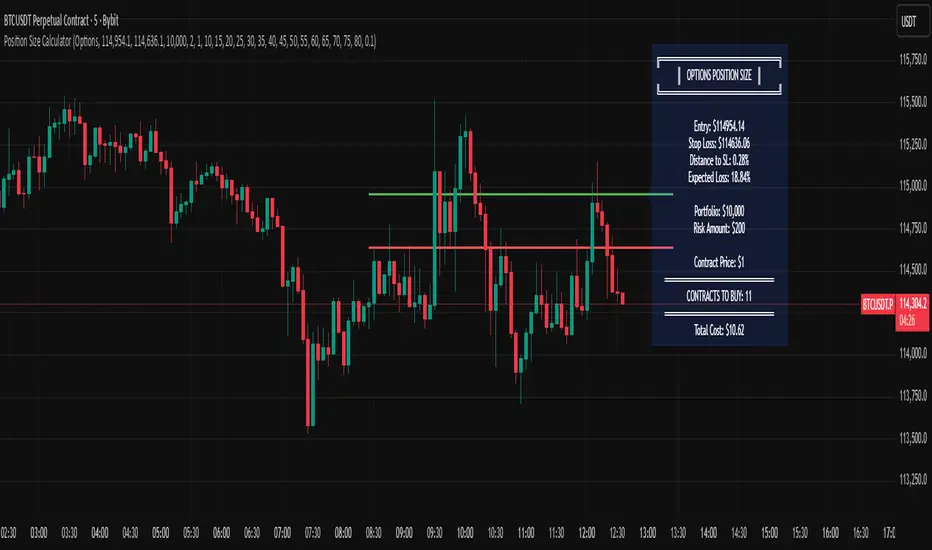
Copter 2.0💡 The indicator is designed for trading on any timeframe and includes a comprehensive system for determining entry and exit points based on technical analysis, price and volume.
📊 In the new version of Copter 2.0, the take profit and stop loss functions have been added
Let's analyze its key components:
✔️ Trend levels and extremes:
- The indicator determines local highs and lows for a certain period.
- the breakdown of these levels serves as a signal to open positions.
- the High-Low price dynamics analysis method is used to find key entry points.
✔️ Volumes:
-The indicator uses a configurable volume threshold to filter out candles with low volume and display only those with significant volume.
- the algorithm analyzes market data and sets an entry signal (opening a trade) and exit (profit taking/closing a position)
📍 Therefore, whether you are a beginner or an experienced trader, the indicator can help you stay ahead of the game and make more informed trading decisions.
📍 As a result, the trader can be sure that the signal is based on data analysis.
A long or short position can be stopped with either a profit or a small loss without prejudice to the potential profit.
✔️ Signal filtering:
- volume and volatile indicators are used to confirm the trend
- if a volume or volatility filter does not confirm the breakdown, the input signal is ignored
- analysis of moving averages of volumes and ATR is used
✔️ The use of the RSI in overbought and oversold analysis:
- the RSI indicator analyzes the strength of the current trend
- if the RSI exceeds 70, exit from a long position is possible
- if the RSI falls below 30, exit from a short position is possible
✔️ The use of EMA 20 and EMA 200
is additional moving average data that determines the current trend and the trend on higher timeframes.
- the main idea is that when they cross, we can see a change in trend movement and determine the general mood at the moment, based on which signals appear to open/close a deal.
- also, the indicator analyzes the past movement, thus determining the future direction
- based on the opening and closing of the past days, weeks, months.
✔️ Stop loss and risk management
- when entering a trade, a dynamic stop loss is set based on the percentage price change
- exit the position is carried out when a stop loss or a signal from the RSI is reached.
- it helps to minimize losses and protect profits
The market is unstable, and it is impossible to know what awaits it in the future.
The only way to manage risk is to limit the loss by setting a stop loss at 1% - 2% of the entry point.
It is recommended to set the profit in the ratio 1:1, 1:2,1:3, with partial fixation of 40%, 30%, 30% or wait for the indicator signal (TP)
We recommend fixing positions in parts. There will be a signal in the opposite direction when the volume is released.
To match the risk of the transaction, we recommend that you do not enter with high leverage.
Trade only with the amount that you are willing to lose.
With increased volatility in the market and flat, the indicator can give many signals.
After a strong fall or growth, we recommend not to open positions, because the probability of a flat is high.
✔️ Visualization of entry and exit points
- Entry points (long and short) are graphically displayed. green - long, orange - short
- stop loss levels are marked for clarity of risk management
✔️Recommendations for working with the indicator!
Entry/exit is performed on the next candle after the candle with the signal (buy/sell)
All timeframes and any trading pairs are used (when selecting settings for each one)
The indicator combines several methods of technical analysis:
- work with support and resistance levels
- filtering of signals based on volumes and volatility
- Overbought and oversold analysis using the RSI
- automatic risk management through stop loss
This approach makes the indicator a useful tool for short-term trading and active scalping.
❗️ NO REPAINT ! ❗️
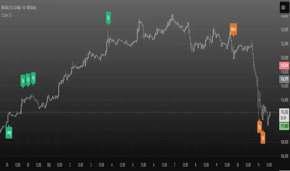
15-Min RSI Scalper [SwissAlgo]15-Min RSI Scalper
Tracks RSI Momentum Loss and Gain to Generate Signals
-------------------------------------------------------
WHAT THIS INDICATOR CALCULATES
This indicator attempts to identify RSI directional changes (RSI momentum) using a step-by-step "ladder" method. It reads RSI(14) from the next higher timeframe relative to your chart. On a 15-minute chart, it uses 1-hour RSI. On a 5-minute chart, it uses 15-minute RSI, and so on.
How the ladder logic works:
The indicator doesn't track RSI all the time. It only starts tracking when RSI crosses into potentially extreme territory (these are called "events" in the code):
For sell signals : when RSI crosses above a dynamic upper threshold (typically between 60-80, calculated as the 90th percentile of recent RSI)
For buy signals : when RSI crosses below a dynamic lower threshold (typically between 20-40, calculated as the 10th percentile of recent RSI)
Once tracking begins, RSI movement is divided into 2-point steps (boxes). The indicator counts how many boxes RSI climbs or falls.
A signal generates only when:
RSI reverses direction by at least 2 boxes (4 RSI points) from its extreme
RSI holds that reversal for 3 consecutive confirmed bars
Example: Dynamic threshold is at 68. RSI crosses above 68 → tracking starts. RSI climbs to 76 (4 boxes up). Then it drops back to 72 and stays below that level for 3 bars → sell signal prints. The buy signal works the same way in reverse.
-------------------------------------------------------
SIGNAL GENERATION METHODOLOGY
Sell Signal (Red Triangle)
RSI crosses above a dynamic start level (calculated as the 90th percentile of the last 1000 bars, constrained between 60-80)
Indicator tracks upward progression in 2-point boxes
RSI reverses and drops below a boundary 2 boxes below the highest box reached
RSI remains below that boundary for 3 confirmed bars
Red triangle plots above price
Reset condition: RSI returns below 50
Buy Signal (Green Triangle)
RSI crosses below a dynamic start level (10th percentile of last 1000 bars, constrained between 20-40)
Indicator tracks downward progression in 2-point boxes
RSI reverses and rises above a boundary 2 boxes above the lowest box reached
RSI remains above that boundary for 3 confirmed bars
Green triangle plots below price
Reset condition: RSI returns above 50
-------------------------------------------------------
TECHNICAL PARAMETERS
All parameters are hardcoded:
RSI Period: 14
Box Size: 2 RSI points
Reversal Threshold: 2 boxes (4 RSI points)
Confirmation Period: 3 bars
Reset Level: RSI 50
Sell Start Range: 60-80 (dynamic)
Buy Start Range: 20-40 (dynamic)
Lookback for Percentile: 1000 bars
Note: Since the code is open source, users can modify these hardcoded values directly in the script to adjust sensitivity. For example, increasing the confirmation period from 3 to 5 bars will produce fewer but more conservative signals. Decreasing the box size from 2 to 1 will make the indicator more responsive to smaller RSI movements.
-------------------------------------------------------
KEY FEATURES
Automatic Higher Timeframe RSI
When applied to a 15-minute chart, the indicator automatically reads 1-hour RSI data. This is the next standard timeframe above 15 minutes in the indicator's logic.
Dynamic Adaptive Start Levels
Sell signals use the 90th percentile of RSI over the last 1000 bars, constrained between 60-80. Buy signals use the 10th percentile, constrained between 20-40. These thresholds recalculate on each bar based on recent data.
Ladder Box System
RSI movements are tracked in 2-point boxes. The indicator requires a 2-box reversal followed by 3 consecutive bars maintaining that reversal before generating a signal.
Dual Signal Output
Red down-triangles plot above price when the sell signal conditions are met. Green up-triangles plot below the price when buy signal conditions are met.
-------------------------------------------------------
REPAINTING
This indicator does not repaint. All calculations use "barstate.isconfirmed" to ensure signals appear only on closed bars. The request.security() call uses lookahead=barmerge.lookahead_off to prevent forward-looking bias.
-------------------------------------------------------
INTENDED CHART TIMEFRAME
This indicator is designed for use on 15-minute charts. The visual reminder table at the top of the chart indicates this requirement.
On a 15-minute chart:
RSI data comes from the 1-hour timeframe
Signals reflect 1-hour momentum shifts
3-bar confirmation equals 45 minutes of price action
Using it on other timeframes will change the higher timeframe RSI source and may produce different behavior.
-------------------------------------------------------
WHAT THIS INDICATOR DOES NOT DO
Does not predict future price movements
Does not provide entry or exit advice
Does not guarantee profitable trades
Does not replace comprehensive technical analysis
Does not account for fundamental factors, news events, or market structure
Does not adapt to all market conditions equally
-------------------------------------------------------
EDUCATIONAL USE
This indicator demonstrates one approach to momentum reversal detection using:
Multi-timeframe analysis
Adaptive thresholds via percentile calculation
Step-wise momentum tracking
Multi-bar confirmation logic
It is designed as a technical study, not a trading system. Signals represent calculated conditions based on RSI behavior, not trade recommendations. Always do your own analysis before taking market positions.
-------------------------------------------------------
RISK DISCLOSURE
Trading involves substantial risk of loss. This indicator:
Is for educational and informational purposes only
Does not constitute financial, investment, or trading advice
Should not be used as the sole basis for trading decisions
Has not been tested across all market conditions
May produce false signals, late signals, or no signals in certain conditions
Past performance of any indicator does not predict future results. Users must conduct their own analysis and risk assessment before making trading decisions. Always use proper risk management, including stop losses and position sizing appropriate to your account and risk tolerance.
MIT LICENSE
This code is open source and provided as-is without warranties of any kind. You may use, modify, and distribute it freely under the MIT License.
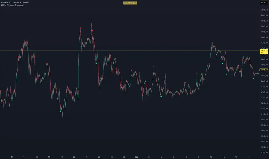
TRP Stop-Loss_Trailing SL# TRP Stop-Loss Indicator
## Overview
The TRP (True Range Percentage) Stop-Loss indicator is an advanced volatility-based stop-loss tool that provides dynamic position protection based on market volatility. Unlike traditional ATR-based indicators, TRP calculates volatility as a percentage of price, offering superior adaptability across different price ranges and market conditions.
## What is TRP and Why It's Superior to ATR
### TRP (True Range Percentage)
TRP calculates the true range as a percentage of the closing price, providing a **normalized volatility measure**. The formula is:
```
TRP = (True Range / Close) × 100
```
### Key Advantages of TRP over ATR:
1. **Price-Normalized Volatility**: TRP automatically adjusts for different price levels, making it equally effective whether you're trading a $10 stock or a $1000 stock.
2. **Percentage-Based Risk**: TRP gives you direct percentage risk values, making position sizing and risk management more intuitive.
3. **Better Cross-Market Comparison**: Unlike ATR, TRP allows you to compare volatility across different instruments on an equal basis.
4. **Adaptive to Market Conditions**: TRP naturally scales with price movements, providing more relevant stop-loss levels during trending markets.
5. **Consistent Risk Exposure**: Maintains consistent percentage risk regardless of the underlying asset's price level.
## Indicator Features
### 🎯 **Dual Stop-Loss System**
- **Long SL**: Red line below price for long positions
- **Short SL**: Blue line above price for short positions
- Independent control for each direction
### ⚙️ **Advanced Calculation Options**
#### **Multiple TRP Calculation Sources:**
- **Current Candle**: Uses real-time running candle data
- **Previous Close**: Uses completed candle data (default)
- **Last Green Candle**: For longs - uses TRP from the most recent bullish candle
- **Last Red Candle**: For shorts - uses TRP from the most recent bearish candle
#### **Independent Multipliers:**
- Separate multiplier controls for long and short stop-losses
- Adjust risk levels independently (0.1x to 10x+ range)
- Fine-tune stop-loss distance based on your risk tolerance
### 📊 **Visual Customization**
- **Line Styles**: Solid, dashed, or dotted lines
- **Custom Colors**: Separate color controls for long/short SL
- **Line Width**: Adjustable thickness (1-10)
- **Extension**: Customizable projection bars to the right
### 🏷️ **Smart Labeling System**
- **Value Display**: Shows exact SL price on the right side of lines
- **Toggle Control**: Enable/disable labels as needed
- **Size Options**: 5 different label sizes (tiny to huge)
- **Color Coordination**: Labels match their respective line colors
### ⏰ **Multi-Timeframe Support**
- Calculate TRP on any timeframe while viewing on another
- Default: Daily TRP calculation for intraday charts
- Maintains calculation integrity across timeframe switches
## How to Use
### Basic Setup:
1. Add the indicator to your chart
2. Select your preferred timeframe for TRP calculation
3. Choose calculation source for long and short positions
4. Adjust multipliers based on your risk tolerance
### Risk Management Applications:
- **Conservative**: Use 0.5-0.8 multipliers for tighter stops
- **Standard**: Use 1.0 multiplier for normal volatility-based stops
- **Aggressive**: Use 1.2-2.0 multipliers for wider stops in volatile markets
### Advanced Strategies:
- **Trend Following**: Use "Last Green/Red Candle" sources to adapt to momentum changes
- **Breakout Trading**: Use "Current Candle" for real-time stop adjustments
- **Swing Trading**: Use "Previous Close" for stable, confirmed levels
## Key Benefits
✅ **Dynamic Adaptation**: Automatically adjusts to changing market volatility
✅ **Percentage Risk Control**: Direct percentage-based risk management
✅ **Multi-Strategy Compatible**: Works with scalping, day trading, and swing trading
✅ **Visual Clarity**: Clean, professional chart display with customizable appearance
✅ **Real-Time Updates**: Instant recalculation when settings change
✅ **No Overlapping Lines**: Smart line management prevents chart clutter
## Best Practices
1. **Backtest First**: Test different multiplier settings on historical data
2. **Market Adaptation**: Adjust multipliers based on current market volatility regime
3. **Combine with Other Signals**: Use TRP stops with your existing entry signals
4. **Position Sizing**: Use TRP percentage values for consistent position sizing
5. **Regular Review**: Periodically review and adjust settings based on performance
## Technical Specifications
- **Pine Script Version**: v6
- **Overlay**: Yes (draws directly on price chart)
- **Calculations**: Based on 50-period EMA of TRP values
- **Updates**: Real-time with automatic line management
- **Performance**: Optimized for fast execution and minimal lag
This indicator is ideal for traders who want professional-grade, volatility-adaptive stop-loss management with the flexibility to fine-tune risk parameters across different market conditions and trading styles.
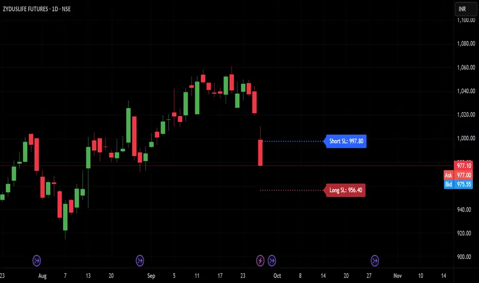
SP2L Pour Samadi Indicator [TradingFinder] Spike 2 Legs PA🔵 Introduction
The SP2L (Spike–2Leg) strategy, designed by Mohammad Ali Poursamadi, an international Iranian trader, is a simple yet powerful price action setup developed to identify precise entry points following sharp market movements.
A Spike refers to a sudden and rapid move in the market, usually triggered by a heavy flow of orders in one direction. This sharp movement creates an Imbalance between buyers and sellers. Since the market does not have time to trade evenly during such moves, it generates Inefficiency on the chart.
The direct result of a spike is usually the formation of a Fair Value Gap (FVG) — a space between candles indicating that trades were not distributed fairly. In simple terms, the spike is the cause, while Imbalance, Inefficiency, and FVG are its consequences.
🟣 How is a Spike formed?
Big Movement : A spike begins with a sharp and powerful move caused by heavy order flow in one direction.
Imbalance : This move disrupts the balance between buyers and sellers.
Inefficiency : Due to the speed of the move, the market fails to trade efficiently, leaving inefficiency on the chart.
Fair Value Gap (FVG) : The final outcome is a price gap between candles, highlighting unfair distribution of trades.
In SP2L, entries occur right after a spike. The entry logic is based on the structure of each candle’s Higher Lows (HLs) or Lower Highs (LHs).
When a spike occurs and candles consecutively form higher lows or lower highs :
In bullish conditions, each previous low becomes a potential Buy Entry.
In bearish conditions, each previous high becomes a potential Sell Entry.
🔵 How to Use
In the SP2L strategy, entries occur directly within the ongoing strong movement (the spike). A spike forms when heavy order flow pushes the market strongly in one direction, creating several large candles in sequence. This disrupts balance and leaves patterns such as Imbalance and FVG on the chart.
During such moves, the market does not necessarily retrace; instead, it continues strongly in the direction of the spike. The key principle in SP2L is that candles begin forming Higher Lows (HLs) in a bullish spike or Lower Highs (LHs) in a bearish spike. Each HL or LH acts as a potential entry level, but the actual entry only triggers once price returns to retest that level. This allows the trader to enter within a powerful wave while keeping stop-losses clear and risk controlled.
🟣 Bullish SP2L
When a bullish spike occurs, candles consecutively form Higher Lows. Each HL marks a potential entry. The entry is activated when price returns to that HL.
Stop-Loss (SL) : Placed below the candle where the spike originated, usually the lowest point before the sharp move.
Take-Profit (TP) : Defined based on classic risk-to-reward ratios, commonly TP1 = 1:1 and TP2 = 1:2. Stronger trends may allow extended targets.
🟣 Bearish SP2L
When a bearish spike occurs, candles consecutively form Lower Highs. Each LH marks a potential sell entry. The entry is triggered when price returns to retest that LH.
Stop-Loss (SL) : Placed above the candle where the bearish spike started, usually the highest point before the sharp drop.
Take-Profit (TP) : Similar to bullish setups, typically TP1 = 1:1 and TP2 = 1:2, with extended targets possible if bearish momentum continues.
🔵 Settings
🟣 Spike Filter | Movement
Minimum Spike Bars : Defines the minimum number of consecutive candles required for a valid spike.
Movement Power : Enables or disables the momentum-based spike filter.
Movement Power Level : Sets the strength threshold; higher values filter out weaker moves and only detect strong spikes.
🟣 Spike Filter | Gap
Gap Filter : Enables or disables the gap filter.
Gap Type : Selects which type of gap should be detected (All Gaps, Significant, Structural, Major).
🟣 Spike Filter | Doji
Doji Tolerance : Defines whether doji candles are allowed within a spike.
Max Doji Body Ratio : Maximum ratio of body-to-total candle size for classifying a candle as a doji.
Max Doji in Spike Ratio : Maximum percentage of doji candles allowed within a spike.
🟣 Trend Detection
Trend Detection : Enables or disables the trend detection module using dojis.
Max Doji Body Ratio : Maximum body-to-candle ratio used to classify a doji in trend calculations.
Candle Lookback : Number of candles used to calculate doji percentage for trend evaluation.
Max Doji in Trend Ratio : Maximum percentage of doji candles allowed within the lookback window for the trend to be valid.
🟣 Position Management
Stop-Loss Threshold : Enables or disables the stop-loss threshold feature.
Stop-Loss Threshold Value : Defines the value of the stop-loss threshold for risk management.
Risk-Reward Ratio : Sets the desired risk-to-reward ratio (e.g., 1:1 or 1:2).
Include SL Threshold in R:R : Determines whether the stop-loss threshold is included in risk-to-reward calculations.
🟣 Display Settings
Display Mode : Chooses between Setup (showing setups) or Signal (showing trade signals).
Only Display the Last Position : Displays only the most recent position on the chart when enabled.
🔵 Conclusion
The SP2L (Spike–2Leg) strategy, designed by Mohammad Ali Poursamadi, offers a simple yet effective framework for trading strong market flows. Built on the logic of spikes and candle structures (HLs and LHs), it identifies precise entry points directly within the main movement of the market, where risk is clear and reward is logical.
With transparent rules, defined stop-loss placement, and flexible risk management, SP2L proves especially effective in volatile markets such as forex, gold, and indices. Its simplicity makes it practical for both beginner traders and seasoned professionals.
In summary, SP2L helps traders avoid unnecessary complexity by focusing on spikes and consecutive HL/LH formations to capture accurate, low-risk entries.

Margin Cost Calculator Screener - Taylor V1.2# Leverage Position Cost Calculator & Stop Lose Cost Screener #
Designed to provide traders with crucial insights into their leveraged positions directly on the TradingView chart.
Key Features:
> Dynamic Display: Choose to view only the estimated entry cost, or a comprehensive overview including potential losses at specific stop-loss levels, and a custom remark.
> Contract Size Input: Easily specify the contract size for your trades.
> Leverage Level Input: Set your desired leverage level, with helpful tooltips explaining the margin requirements for various leverage ratios (e.g., 25x, 10x, 5x) and an included fee estimate.
> Cost Calculation: Accurately calculates the estimated entry cost for your position based on the current market price, contract size, and leverage.
> Stop-Loss Projections: It projects potential losses for stop-loss orders set at 3% and 5% below the entry price, helping you manage risk effectively.
> Clear Table Visualization: All calculated data is presented in a clean, organized table anchored to the bottom-left of your chart, making it easy to reference at a glance.
> Symbol Identification: Automatically displays the short ticker symbol for the asset you are analyzing.
This tool is invaluable for traders who utilize leverage and need a quick, visual way to understand their financial exposure and potential outcomes before entering or managing a trade.
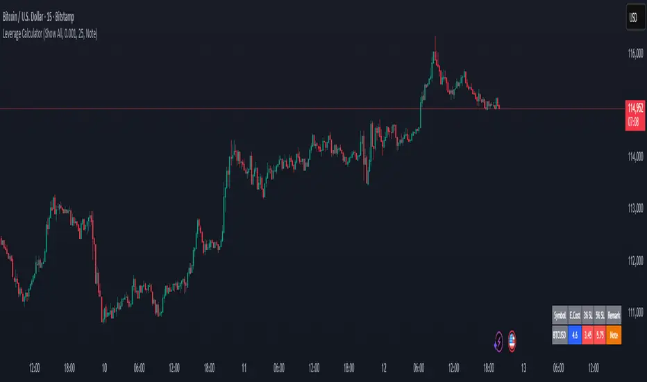
Sniper Swing — Short TF (Clean Signals) [v6]📘 How to Use the Sniper Swing Indicator
1. What It Does
It looks for short-term swing breaks in price.
It uses an oscillator (RSI/Stoch) and swing pivots to confirm moves.
It gives you 3 clear signals only:
BUY → Enter long (expecting price to go up).
Gay bear → Enter short (expecting price to go down).
EXIT → Close your trade (long or short).
Candles also change color:
Green = in a BUY trade.
Red = in a Gay bear trade.
Neutral (gray/none) = no trade.
2. When to Use
Works best on short timeframes (1m–5m) for scalping/intraday.
Use on liquid markets (MES/ES, NQ, SPY, BTC, ETH).
Avoid dead hours with no volume (like overnight futures lull or midday chop).
3. How to Trade With It
A. BUY trade
Wait for a BUY triangle below the candle.
Confirm:
Candle turned green.
Price broke a recent swing high.
Oscillator shows strength (indicator does this for you).
Enter long at the close of that candle.
Place your stop-loss:
At the yellow stop line (auto trailing stop), or
Just below the last swing low.
Stay in while candles are green.
Exit when:
An orange X appears, or
Price hits your stop.
B. Gay bear (short) trade
Wait for a Gay bear triangle above the candle.
Confirm:
Candle turned red.
Price broke a recent swing low.
Oscillator shows weakness.
Enter short at the close of that candle.
Place stop-loss:
At the yellow stop line, or
Just above the last swing high.
Stay in while candles are red.
Exit on an orange X or stop hit.
4. Pro Tips for New Traders
Only take one signal at a time → don’t double dip.
Quality > Quantity: ignore weak, sideways markets. Best signals happen during trends.
Start small: trade micros (MES) or small position sizes.
Use alerts: set TradingView alerts for BUY/Gay bear/EXIT so you don’t miss setups.
Think of the indicator like a navigator: it tells you the likely path, but you’re the driver → always manage risk.
5. Quick Mental Checklist
Signal? (BUY or Gay bear triangle)
Confirmed? (candle color + swing break)
Enter? (on close)
Stop? (yellow line or swing)
Exit? (orange X or stop)
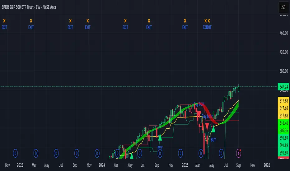
2ATR / Close %Certainly. Here is the English version of the indicator description you requested.
---
### **2ATR Stop-Loss Ratio**
This indicator provides a straightforward calculation of **what percentage a 2ATR (Average True Range) move represents relative to the current price**. It's a specialized tool designed to help traders set dynamic, volatility-based stop-loss levels.
---
### **Purpose of the Indicator**
Many traders use a **2ATR** as their standard for setting a stop-loss, believing it's a good measure of a stock's typical movement. However, it can be difficult to quickly determine the exact percentage a 2ATR drop represents from the current price. This indicator solves that problem by giving you a clear, single number that shows the **anticipated percentage loss before you even enter a position**.
---
### **How It Works**
The indicator is calculated using a simple formula:
**(2 * ATR(20) / Current Price) * 100**
* `ATR(20)`: The Average True Range over the last 20 periods. This period can be customized in the indicator's settings.
* `Current Price`: The closing price at the time of calculation.
---
### **How to Use It**
* **Assess Risk**: A higher number on the indicator means greater volatility, indicating a wider stop-loss range.
* **Set a Stop-Loss**: If the indicator shows **3%**, it means a 2ATR move is roughly a 3% change from the current price. This gives you a clear understanding of the potential loss.
* **Adjust Position Size**: If the potential percentage loss is larger than you're comfortable with, you can use this information to reduce your position size, effectively managing your risk.
This tool is especially useful for trading highly volatile stocks, as it helps you establish a clear and effective risk management strategy.

Position Size CalculatorPosition Size Calculator
This open-source Pine Script® indicator helps traders manage risk by calculating position size, margin, and risk/reward based on account size, leverage, entry, stop-loss, and take-profit. It features a customizable table and optional chart lines/labels for clear trade planning across stocks, forex, crypto, and futures.
What It Does
- Position Size: Computes units to trade based on risk percentage and stop-loss distance, capped by leverage.
- Margin: Calculates initial margin in base currency and USD, with account size percentage.
- Risk/Reward: Shows risk-reward ratio, percentage price movements, and USD gains/losses.
- Visualization: Displays results in a table and optional chart lines/labels with customizable styles.
How It Works
- Precision: Adjusts price formatting using syminfo.mintick for accuracy across assets.
- Calculations: Position size = accountSize * (riskPercent / 100) / |entry - stoploss|, capped by accountSize * leverage / entry. Margin = positionSize / leverage. Risk-reward = |takeprofit - entry| / |stoploss - entry|.
- Display: Table shows metrics; optional lines/labels plot entry, stop-loss, and take-profit with percentage and USD details.
How to Use
- Set Inputs:
1- Account Size (USD): Your capital (e.g., 1000).
2- % Risk per Trade: Risk tolerance (e.g., 1%).
3- Leverage: Broker leverage (e.g., 1x, 10x).
4- Entry, Stop Loss, Take Profit: Trade prices.
5- Show Lines and Labels: Enable chart overlays.
- Customize: Adjust table position, colors, and line styles (Solid, Dashed, Dotted).
- View Results: Table shows position size, margin, and risk/reward. Chart lines/labels (if enabled) display prices, percentages, and USD outcomes.
- Apply: Use metrics for trade execution; modify code for custom features.
Notes
- Ensure valid inputs (entry ≠ stop-loss, both positive) to avoid “N/A”.
- Open-source: Inspect or extend the code for your needs.
- Contact the author via TradingView for feedback.